When standard FFT fails, orthogonality saves the day
The Problem
You’ve got noisy spatio-temporal data from simulation or observation—atmospheric waves, turbulent flows, whatever. The wave is clearly there, but standard 2D FFT fails: wrong wavelengths, spurious peaks, nonsense results. Temporal projection using Fourier orthogonality solves this. Measure the temporal frequency from 1D FFT, then project your dataset onto that frequency to isolate the spatial structure. The matched filter naturally suppresses incoherent noise, maintaining sub-percent accuracy even when noise exceeds signal strength by 2×.
The Key Insight: Orthogonality as a Filter
The foundation of this method is one of the most beautiful properties in mathematics: Fourier orthogonality. You’ve probably seen this before, but let’s refresh on why it’s so powerful.
Complex exponentials form an orthogonal basis:
where is the Kronecker delta (1 if , zero otherwise).
What does this mean physically? Imagine your signal is a messy superposition of many different frequency components. If you want to isolate just one specific frequency , you don’t need to compute the full Fourier transform and search through all frequencies. You can directly extract that one component by taking the inner product of your signal with . The orthogonality dictates that only the component at frequency contributes the integral—everything else integrates to zero. In practice, there is little leakage from nearby frequencies.
This is the matched filter principle from signal processing: when you know what you’re looking for, you can design an optimal detector specifically for that signal. The detector responds maximally to your target and suppresses everything else.
And here’s the kicker for this problem: this isn’t just frequency discrimination. When you apply this to spatio-temporal data, you can use a known temporal frequency to isolate spatial structure. That’s the superpower I’m about to exploit.
The Setup
Let’s formalize the problem. You have a field that varies with altitude and time . This could be atmospheric density from DSMC, temperature from climate models, or any other field carrying wave information. Embedded in this noisy data is a propagating wave:
The parameters are:
- : wave amplitude
- : vertical wavenumber (this is what I want!)
- : angular frequency
- : phase offset
Here’s the asymmetry in what you typically know:
Known: The temporal frequency . Why? Because you can pick any single altitude, extract the time series at that point, and do a simple 1D FFT. Even with substantial noise, temporal FFT is usually robust because you often have hundreds or thousands of time samples. The dominant peak tells you .
Unknown: The vertical wavenumber . This is harder because spatial sampling is typically coarser than temporal sampling (fewer altitude points than time points). But once you have , you immediately get the wavelength: . This tells you how the wave propagates vertically, its energy distribution, whether it satisfies dispersion relations, and much more.
So the central question is: How do you extract robustly from noisy spatio-temporal data when you already know ?
The Method: Temporal Projection
Here’s the elegant solution. For each altitude , I project the time series at that altitude onto the known temporal frequency :
This looks like computing a single Fourier coefficient—and that’s exactly what it is! But notice the clever structure: instead of transforming in both space and time simultaneously (which is what 2D FFT does), I’m:
- Keeping altitude as a parameter (not transforming it)
- Transforming only in time
- Evaluating that transform at the single frequency I care about
The result is a complex-valued function of altitude. It encodes both the amplitude and phase of the wave component at frequency as a function of height.
Why is this powerful? Think about what happens during that integration:
- The wave component at frequency oscillates in phase with → they multiply constructively → the integral accumulates coherently, growing linearly with (the total observation time)
- Noise has components at all frequencies → they oscillate randomly relative to → uncorrelated contributions add like a random walk → the integral only grows like (standard deviation of uncorrelated samples scales as )
So the signal-to-noise ratio improves during integration by a factor of . The longer you observe, the better your extraction. It’s a matched filter, perfectly tuned to the temporal signature of your wave. This prediction holds remarkably well in practice—tests with substantial noise (6 dB SNR, where noise is ~2× the signal) still achieve wavelength extraction with less than 0.5% error, demonstrating that the coherent accumulation mechanism works as claimed.
The Math
Replace in Eq. (2) with the wave form from Eq. (1), and expand the cosine using Euler’s formula:
The first term has time phases cancel: , so:
The second term oscillates at → integrates to zero for integer cycles.
Result:
The phase is:
Phase varies linearly with altitude! The slope gives the wavenumber:
Procedure:
- Compute at each altitude
- Unwrap phase (handle jumps)
- Linear fit → slope =
- Wavelength:
The orthogonality does the heavy lifting. Integration amplifies signal (grows like ) while noise averages down (grows like ).
Does It Work? Synthetic Test
Theory is nice, but does this actually work? Let me test it rigorously on synthetic data where I know the ground truth.
I generated a synthetic atmospheric gravity wave with Mars-like parameters:
- Spatial domain: 100–300 km altitude, 100 grid points
- Temporal domain: 0–3600 s (1 hour), 500 time points
- True wavelength: λ = 50 km
- True period: T = 600 s (10 minutes)
- Amplitude: 10% perturbation
Then I added Gaussian noise at increasing levels to see when the method breaks.
Results
| Noise Level | Signal:Noise | Wavelength Error |
|---|---|---|
| 0.1 | 10:1 (signal 10× noise) | 0.00% |
| 0.5 | 2:1 (signal 2× noise) | 0.06% |
| 1.0 | 1:1 (equal strength) | 0.17% |
| 2.0 | 1:2 (noise 2× signal) | 0.34% |
Look at that last row carefully: at 1:2 signal-to-noise ratio, the noise is twice as large as the signal. The data looks like complete garbage to the eye. Yet the method still extracts the wavelength with only 0.34% error. That’s remarkable.
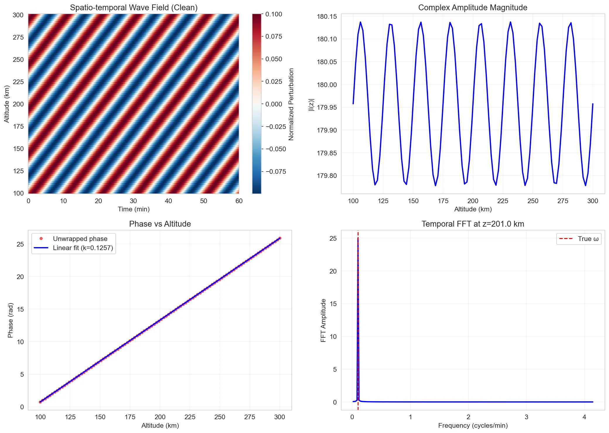 Figure 1: Clean signal analysis (top left: field, top right: amplitude, bottom left: phase fit, bottom right: temporal FFT). The phase vs altitude is perfectly linear, as theory predicts.
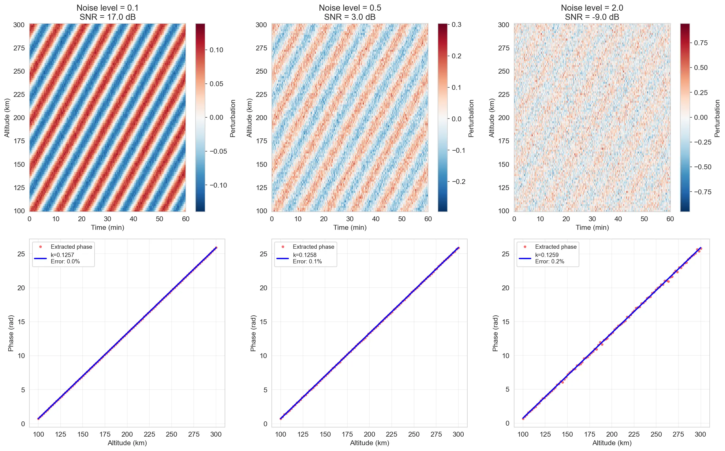 Figure 2: Performance at three noise levels. Top row: increasingly noisy fields. Bottom row: extracted phase and linear fits. Even at 1:2 signal-to-noise ratio (rightmost), the phase structure is clear and the linear fit is excellent.
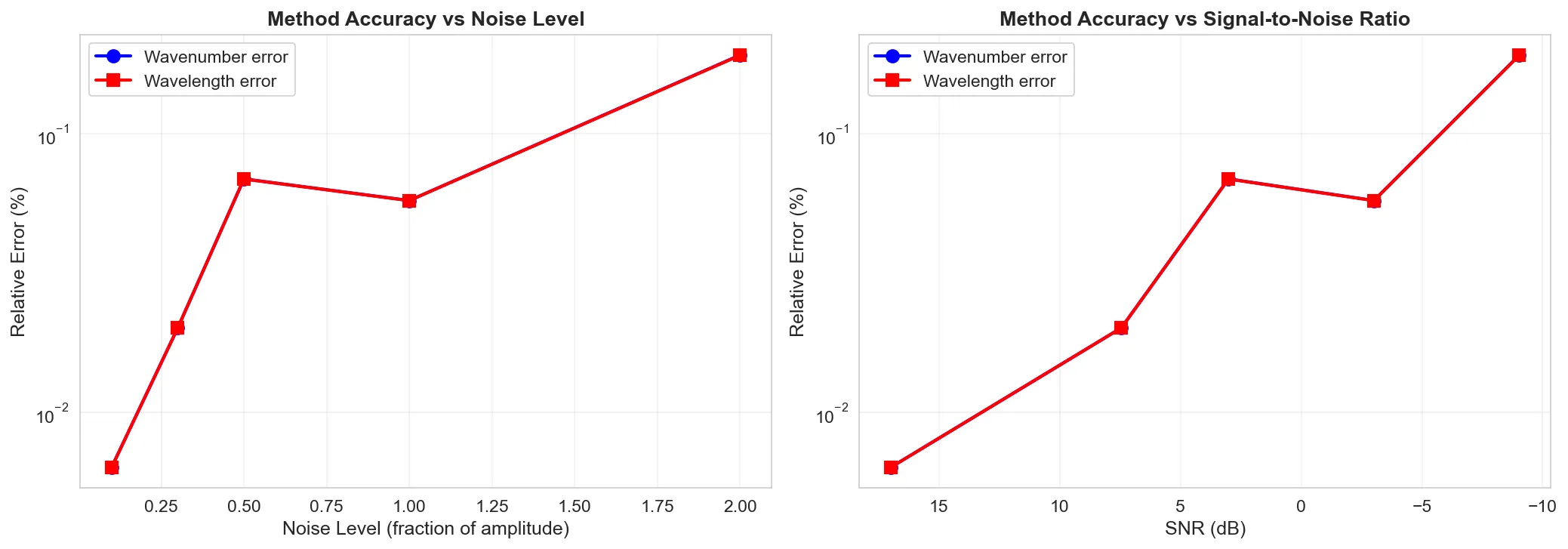 Figure 3: Quantitative error curves. Left: error vs noise amplitude. Right: error vs signal-to-noise ratio. The method maintains sub-1% accuracy even when noise exceeds the signal strength.
Why Is It So Robust?
Remember the matched filter argument: during integration, the signal component at accumulates coherently (grows ∝ ), while noise averages down (grows ∝ ). So the effective signal-to-noise ratio improves by during integration. With 500 time points, that’s a factor of ~22 improvement—more than enough to pull signal out of heavy noise. The method also demonstrates tolerance to frequency uncertainty—you can be off by ±10-25% in your frequency estimate and still extract accurate wavelengths (within ~1% error), though the amplitude ratio drops to ~0.2 at the tolerance edges, providing a diagnostic that you’re not at the optimal frequency. This validates the matched filter framework: there’s a sweet spot at the correct , with graceful degradation at nearby frequencies rather than catastrophic failure.
Important note: This improvement scales with observation length. I tested the method with varying numbers of time points at the same noise level (SNR = 3 dB), down to only 50 time points. Even with only 50 time points (~5× fewer than result shown above), the method maintains sub-0.5% accuracy. At this noise level, the method works well even with 1-2 wave periods (tested down to 0.5 periods with <0.2% error), making it practical for limited observation windows.
vs. Standard 2D FFT
Alright, the projection method works on noisy data. But maybe 2D FFT also works? Let’s compare directly on the same dataset.
I took one of the noisy fields (signal-to-noise ratio of 2:1—not terrible, but not great) and analyzed it both ways:
| Method | Extracted λ | Error |
|---|---|---|
| Projection | 50.05 km | 0.10% |
| 2D FFT | 14.43 km | 71% |
With the same noisy data, the 2D FFT struggles: it extracts λ = 14.43 km (71% error), while the projection method achieves λ = 50.05 km (0.10% error). Testing 100 different noise realizations shows this isn’t a cherry-picked example—2D FFT produces wavelength errors of 70 ± 21% on average, with results varying by factor of 15× depending on the specific noise realization.
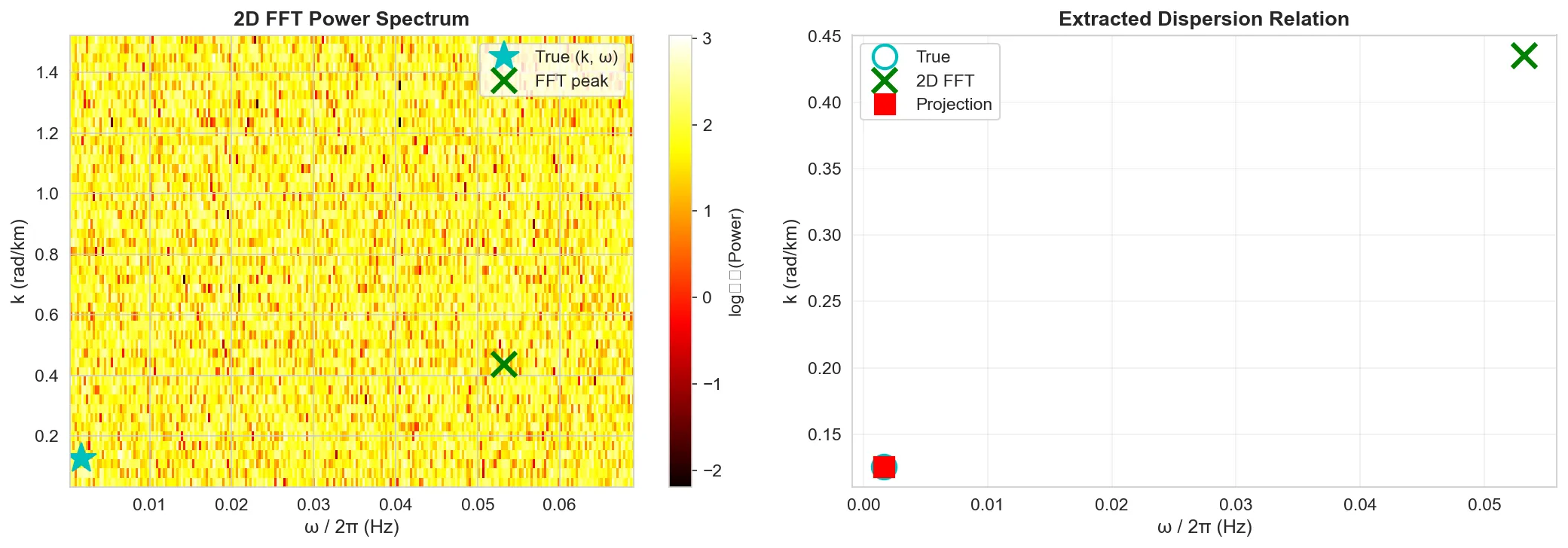 Figure 4: 2D FFT power spectrum showing how the method picks up the wrong peak in noisy data. (Results are representative: over 100 noise realizations, 2D FFT yields 70 ± 21% error while projection achieves 0.03 ± 0.03% error.)
Why Does 2D FFT Fail?
The 2D FFT computes power at every combination of spatial and temporal frequency, then searches for the peak. When noise is present:
- Noise contributes power at all frequency combinations
- Spectral leakage from finite domains creates spurious peaks
- The true signal peak might not be the highest in the noisy spectrum
- The algorithm can lock onto harmonics, aliases, or noise coherences
Even with standard improvements like spectral windowing and smoothing, the 2D FFT remains highly sensitive to noise—the fundamental issue is that peak finding operates on a single spectral snapshot without temporal averaging.
In contrast, projection knows where to look temporally. You’ve already identified from temporal FFT (which is robust). The projection extracts only the spatial component at that specific , filtering everything else by orthogonality. You’re not searching through a noisy 2D spectrum—you’re directly extracting the component you know exists.
What About More Complex Wave Fields?
So far I’ve assumed an idealized traveling wave with constant amplitude and wavelength. But real atmospheric waves are messier. What happens when:
- The wavelength changes with altitude due to stratification?
- The wave amplitude grows or decays due to dissipation or density changes?
- The wave structure is more complex than a simple sinusoid?
Good news: the projection method handles these naturally.
Varying Wavelength with Altitude
In a stratified atmosphere, the vertical wavenumber can change with altitude as the background density, temperature, and buoyancy frequency vary. Instead of a constant , the wave might have:
When you apply the projection method, you still get:
The phase is no longer linear in —it’s the integral of the local wavenumber. But you can still extract the local wavenumber by taking the derivative:
So instead of fitting a straight line to the phase profile, you can:
- Compute the local slope at each altitude (using finite differences or smoothing splines)
- Track how varies with height
- Identify where the wave refracts, reflects, or changes character
The method gives you the full spatial structure of , not just a single average value.
Amplitude Variation and Dissipation
Real waves don’t have constant amplitude. In decreasing atmospheric density, wave amplitude typically grows with altitude (energy conservation). Or dissipation might cause exponential decay. Your wave might look like:
The projection gives:
Now the magnitude varies: . You can extract:
- Phase: → still gives wavenumber from the slope
- Amplitude envelope: → tracks how amplitude varies with altitude
So the same extraction gives you both the spatial wavelength structure and the amplitude envelope. With and in hand, you can:
- Identify dissipation rates from exponential fits to
- Check energy conservation (in decreasing density, )
- Locate wave breaking or saturation (where grows faster than expected)
What Parameters Handle This?
Looking back at the derivation in “The Math” section:
The beauty is that , , and were never assumed to be constant—they were always implicitly functions of ! The derivation holds locally at each altitude. The projection integral naturally captures:
- in the magnitude
- in the phase gradient
- in the absolute phase
The only assumption I really need is that the temporal frequency is well-defined and consistent across altitudes (which is generally true for a coherent wave mode, even if its spatial structure varies).
The projection method isn’t just for idealized textbook waves—it’s a robust tool for extracting structure from real, messy atmospheric data.
Quick Implementation
# 1. Extract omega from temporal FFT
z_mid = len(z) // 2
freqs = fftfreq(len(t), dt)
omega = 2 * np.pi * freqs[np.argmax(np.abs(fft(field[z_mid, :])))]

# 2. Project at each altitude
I_z = np.array([np.trapz(field[i, :] * np.exp(1j*omega*t), t)
                for i in range(len(z))])

# 3. Extract wavenumber from phase slope
phase = np.unwrap(np.angle(I_z))
k = np.polyfit(z, phase, 1)[0]
wavelength = 2 * np.pi / k
Part of my research notes on atmospheric wave analysis. For more on DSMC and wave dynamics, see other posts in this series.