Wave-Driven Momentum Transport in Molecular Gas Simulations

Understanding wave behavior in simulation data is a complex but fascinating challenge. In my research, I’ve been particularly focused on quantifying momentum transfer caused by traveling waves, a topic that has garnered significant interest in the field.

To establish a solid theoretical foundation for calculating these quantities, I turned to Bird’s 1994 textbook, a comprehensive resource for DSMC (Direct Simulation Monte Carlo) kinematic modeling and theory. Let me share some fundamental concepts about molecular gas behavior in these simulations.

Macroscopic Stream Velocity

The macroscopic stream velocity $\bm{c_{0}}$ , analogous to wind in atmospheric systems, represents the average velocity of all molecules $\bm{c_i}$ within a small region of gas. It can be expressed in two equivalent ways:

\begin{align*} \bm{c_{0}} &= \frac{1}{n} \sum_{i=1}^{n} \bm{c_{i}} = \overline{\bm{c}} \quad \text{or} \\ \bm{c_{0}} &= \frac{1}{\rho} \sum_{i=1}^{j} m_i n_i \overline{\bm{c}_i} \end{align*}

Here, $\rho=\left(\sum_{i=1}^j m_i N_{p, i} W_{p, i}\right) / V_{\text {cell }}$ represents the total mass density of all species in the cell, and $\overline{\bm{c}_i}=\left(\sum_{k=1}^{N_{p, i}}\left(\bm{c}_{p, i}\right)_k\right) / N_{p, i}$ is the average of sampled instantaneous velocity vectors for all particles of species $i$ in the cell.

Peculiar Velocity

The peculiar velocity $\bm{c'}$ (also known as random velocity or thermal velocity $\bm{v_{th}}$ in HARRAH) describes the motion of individual molecules relative to the mean flow:

\bm{c'} = \bm{c} - \bm{c_{0}}

Flux Vector Analysis

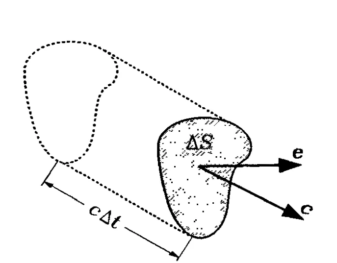
A flux vector quantifies the transport of various properties through a unit area in a gas per unit time. Whether measuring number flux (molecules passing through) or mass flux, the vector indicates both direction and magnitude of the flow. Mathematically, it’s expressed as:

n\sum \left[(\Delta n / n) Q \bm{c} \cdot \bm{e}\right] = n \overline{Q \bm{c}}

where $\bm{e}$ is the unit vector normal to the element area $\Delta S$ .

Mass Transport

For mass transport, setting $Q$ equal to molecular mass gives:

n m \overline{\bm{c'}} \quad \text{or} \quad \rho \overline{\bm{c'}}

Momentum Transport

For momentum transport ( $Q = m \bm{c'}$ ), we obtain the pressure tensor:

\bm{p_{tensor}} = n m \overline{\bm{c'}\bm{c'}} = \rho \overline{\bm{c'}\bm{c'}}

The pressure tensor components can be written concisely as:

p_{ij} = \rho \overline{c'_i c'_j}

Temperature Relations

The translational kinetic temperature $T_{tr}$ relates directly to thermal velocity:

T_{tr} = \frac{m \overline{\bm{c'}^2}}{3 k_B} = \frac{m \left(\overline{c'^2_1} + \overline{c'^2_2} + \overline{c'^2_3}\right)}{3 k_B}

Component-wise:

T_{tr,i} = \frac{m \overline{c_i'^2}}{k_B}

These temperatures connect to pressure tensor components:

p_{ii} = \rho \overline{c'_i c'_i} = \rho \overline{c'^2_i} = n k_B T_{tr,i}

Practical Applications in HARRAH

In HARRAH simulations, we sample radial $v_{r,i}$ , azimuthal $v_{\phi,i}$ , and zenith $v_{\theta,i}$ speeds for each particle species $i$ . These sampled values correspond to the $\overline{c_i}$ in our equations. Using these measurements, we can derive the bulk flow contribution to thermal temperature:

\bm{c_0}^2 = \overline{\bm{c}^2} - \frac{3 k_B T_{tr}}{m}

This relationship helps us understand the mean flow’s influence on the pressure tensor:

p_{ij} = \rho \left(\overline{c_i c_j} - c_{0,i} c_{0,j}\right)

Finally, we can express the scalar pressure $p$ in terms of average velocity components:

p = \frac{1}{3} \rho \left(\overline{\bm{c}^2} - \bm{c_0}^2\right) = n k_B T_{tr}

Leading to the crucial relationship:

\begin{align*} \frac{1}{3}\rho \bm{c_0}^2 = \frac{1}{3} \rho \overline{\bm{c}^2} - p = \frac{1}{3} \rho \overline{\bm{c}^2} - n k_B T_{tr} \end{align*}

This final expression reveals the mean flow’s contribution to both scalar pressure and the pressure tensor, providing valuable insights into momentum transport in our simulation system.