How Often Will Your Particle Classifier Cry Wolf?
Lab accuracy tells you how often a model is right. A sponsor wants to know how often it is wrong, per day.
Not long ago an interviewer asked me a question that has stuck with me since. I had just walked through my semi-supervised classifier for single-particle mass spectra, the one that sorts aerosol particles into a 20-class laboratory library under label scarcity and class imbalance, and he asked: what else have you applied it to? I answered with datasets. What he was really asking, I think, was whether the work is a method that ran once or a capability you can point at a new problem. So I went and pointed it at one.
Here is the problem. A recent Defense Threat Reduction Agency call for a bioaerosol trigger asks for a detection probability of at least 90% for relevant agents, no more than one false alarm per 24 hours in a complex background, a response time under 10 seconds, and demonstrated rejection of at least three common interferents: diesel soot, Arizona road dust, and pollen. Read that list again and notice what is missing. There is no accuracy, no F1 score, no confusion matrix. There is not even a method. There is a rate, a probability, and a clock, and the program office will fund whoever can move those numbers. Almost nobody who publishes aerosol classifiers reports them, which means the number a sponsor needs is the number the literature leaves out.
The Translation Nobody Writes Down
A classifier reports a label and a posterior for one particle: the probability it assigns to each of its 20 classes, given that particle’s spectrum. I use the word the way machine learning does, not the way a Bayesian would. These are model outputs: a softmax for the networks, a fitted probability mapping for the SVMs. An instrument in the field sees a stream of particles and has to decide, continuously, whether to ring the bell. The bridge between those two things is short enough to fit on one line. If every particle the classifier flags as an agent raises an alarm, then
where is the per-particle false-positive fraction (the share of harmless background particles scored as agent) and is the number of background particles the instrument sees in 24 hours. Nothing about this is deep. What makes it brutal is the size of .
On the background day I used, which I describe below, particles arrived at 130,687 per 24 hours of sampling. Plug that in and the requirement of one false alarm per day demands a per-particle false-positive fraction of about , or one wrong call in 130,000 particles. A classifier that is 99.99% specific per particle, a number that would look spectacular in any paper, still rings the bell about 13 times a day. That’s the whole problem in one sentence: a per-particle error rate that looks excellent in the lab can still be orders of magnitude away from the per-day rate a fielded system is specified in. On this day, my four models flag between 0.05% and 0.15% of background particles as bacterial, which is 60 to 200 times more than a one-per-day specification allows.
There is a second, quieter consequence. My entire background day contains 14,478 particles, so the smallest nonzero false-positive fraction it can even resolve is one in 14,478. The requirement sits about 9× below that floor. No amount of threshold tuning on this dataset can demonstrate compliance, and I would rather say that up front than have a reviewer say it for me.
The Setup
You need two ingredients to measure a false-alarm rate honestly: a real background with timestamps, and a guarantee that nothing in it is the thing you are trying to detect. I had both, somewhat by accident. My classifier work came with a “blind” pool of 14,478 unlabeled particles that turned out not to be an undated bag of spectra but a single instrument day with real arrival times: the blind sampling period of the FIN-01 ice nucleation workshop at the AIDA chamber, a published experiment (Shen et al., 2024) whose single-particle spectra are openly archived with Christopoulos et al. (2018). The chamber held a three-component mixture of secondary organic aerosol, Argentinian agricultural soil dust, and soot, and its reference composition contains no biological material. That makes the day bio-free by design (ruling out carryover from earlier chamber use is still on my list), so every biological call any model makes on it is a false alarm. It is not a simple background, though. Soil dust carries its own organic matter, and the chamber produced SOA-coated dust particles, so organic signatures show up on abiotic particles, which is exactly the kind of complex background a trigger has to survive. One more detail matters: the soot was produced by a different generation route than the only soot in my training library, and most of it was likely too small for the instrument to detect at all. The sampled stream is therefore dominated by SOA, soil dust, and their mixtures, and whatever soot did get through has no correct label available.
I ran four classifiers I had already built for that work: a supervised support vector machine, a self-training SVM, a stacked-autoencoder classifier, and a Mean Teacher network. I did not retrain anything. Each model’s full 20-class posterior was already frozen for every particle, so the benchmark is purely an alarm layer: a set of functions that turn posteriors into a score per particle, run decision rules over the time-ordered stream, and count alarms. The primary agent target is bacterial (the library’s Bacteria and Snomax classes, the latter being inactivated Pseudomonas syringae), with all five biological classes as a secondary target. Every rate carries an exact 95% Poisson interval.
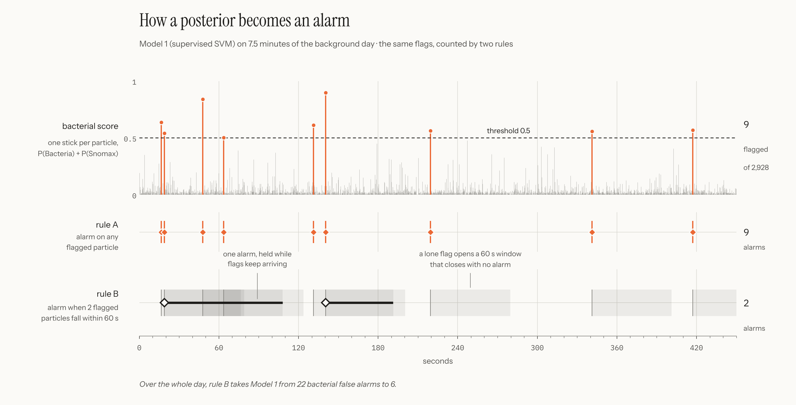 Figure 1: How a posterior becomes an alarm, on 7.5 minutes of the real background stream scored by the supervised SVM. Top: each particle’s bacterial score, the summed posterior on Bacteria and Snomax. Middle: alarming on any flagged particle. Bottom: alarming when two flagged particles fall within 60 seconds; shaded boxes are the 60-second windows each flag opens, and black bars are the time the alarm condition holds.
Figure 1 shows what that layer does on a short stretch of the real stream. Each of the 2,928 particles in those 7.5 minutes gets a bacterial score, and nearly all of them sit close to zero. Nine cross the 0.5 threshold. The simplest rule, alarm on any flagged particle, turns those nine flags into nine alarms. A persistence rule asks for corroboration instead: it alarms only when two flagged particles land within 60 seconds of each other. Because an alarm is the rising edge of that condition, a burst of flags counts once, and a lone flag opens a window that closes without anyone being paged. On this stretch, the same nine flags become two alarms. The benchmark runs the rest of the rules a system engineer would actually consider in the same way: longer windows (3 within 300 s), of the last particles, and an exponentially weighted moving average on the flagged fraction.
The first thing the benchmark did was correct my own plan. I had been dividing alarm counts by the 8.16-hour wall-clock span of the day. But the instrument only recorded particles for 2.66 hours of that span; the rest is eight gaps longer than ten minutes where nothing was sampled. Dividing by the wall clock understated every rate by a factor of 3.07. It’s an easy mistake, and it’s exactly the kind of mistake that makes a system look three times better than it is.
Same Accuracy, Different Alarms
On the 1,868-particle laboratory development set, the four models are nearly indistinguishable: accuracies of 0.903, 0.900, 0.912, and 0.906, a spread of 1.2 percentage points. If you were choosing a model from the manuscript’s tables, you would pick the stacked autoencoder and feel fine about it.
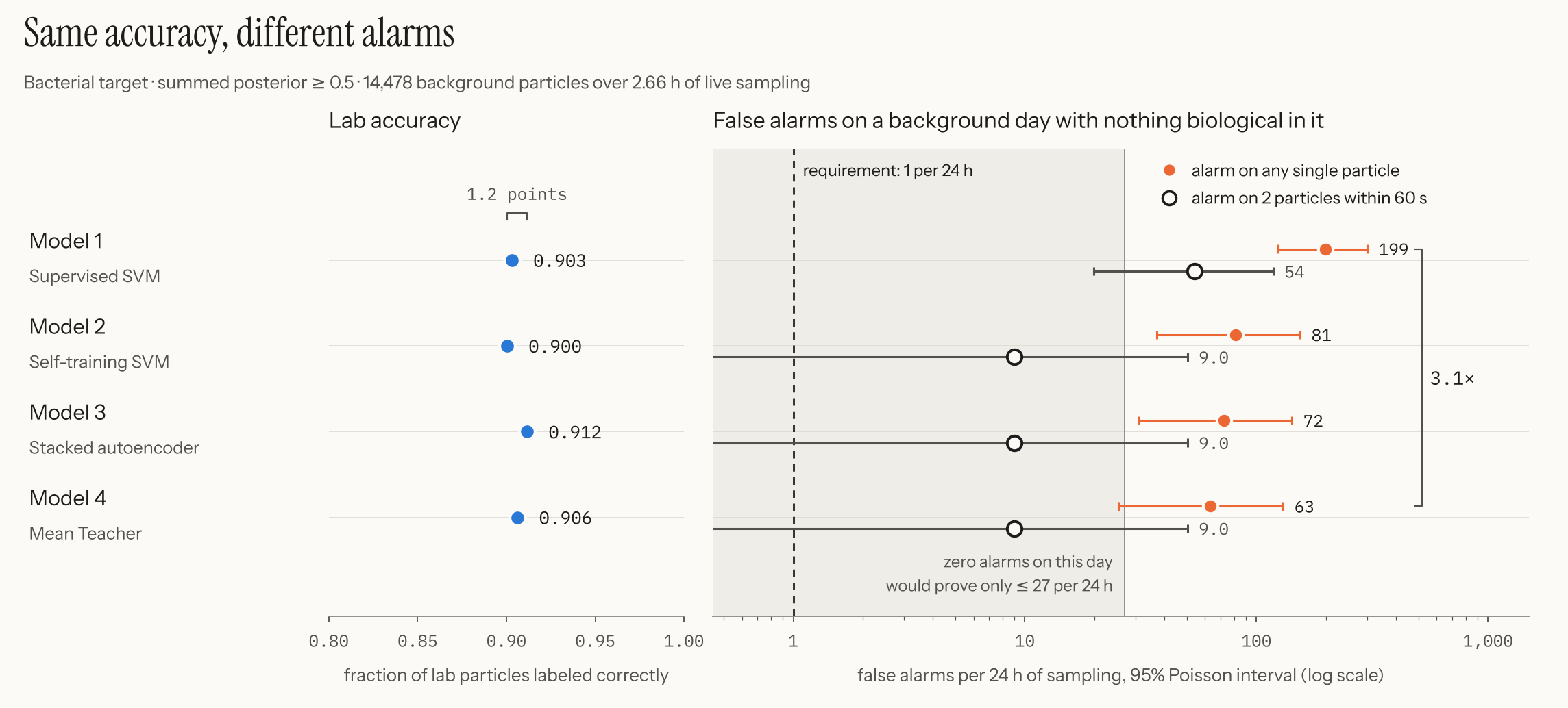 Figure 2: Lab accuracy versus false alarms on a bio-free background day. Left: decision-rule accuracy on the laboratory development set. Right: bacterial false alarms per 24 hours of live sampling, summed posterior at threshold 0.5, with exact 95% Poisson intervals. Filled points alarm on any single flagged particle; open points require two flagged particles within 60 seconds. The shaded region is everything this 2.66-hour day is too short to certify.
Now put them on the background day. Alarming on any single flagged particle, the supervised SVM raises 22 bacterial false alarms, which is 199 per 24 hours, while the Mean Teacher raises 7, or 63 per 24 hours. That is a 3.1× spread in the metric the sponsor cares about, hiding underneath a 1.2-point spread in the metric the manuscript reports. On the broader any-biological target, the same pattern holds: 54 alarms against 36. The model the tables rank first is not the one that cries wolf least.
Then change the rule instead of the model. Requiring two flagged particles within 60 seconds cuts the false-alarm rate of the three semi-supervised models by 7–9×, from 63–81 down to 9 per 24 hours each, and cuts the supervised SVM by 3.7×. In other words, the alarm rule moves the answer more than the model choice does. A program office choosing between classifiers on their lab accuracy is optimizing the smaller knob. Even the scoring choice matters more than you would guess: if the supervised SVM’s score is defined by whether a bacterial class wins the argmax rather than by the summed bacterial probability, its single-particle false alarms jump from 22 to 80, because its Snomax calls carry diffuse posteriors that mostly sit below 0.5.
There is an honest limit to this comparison. Under the 2-in-60-s and 3-in-300-s rules, the three semi-supervised models raise one or two alarms each, which is statistically indistinguishable from each other and from zero on a day this short. Every one of those alarms falls inside a single window late in the day, about nine minutes long, where all four models make bacterial calls at once. If that window turns out to be a real biological intrusion, those models made no bacterial false alarms under persistence at all; if it is an interferent, it is their entire false-alarm record. That window’s identity is a question I still need to settle with the people who ran the experiment, and the benchmark reports it as its own named event rather than averaging it into the day.
The Interferent Nobody Trained For
The more revealing result is not the bacterial target at all. It is what happens when the models meet material that was never in their library.
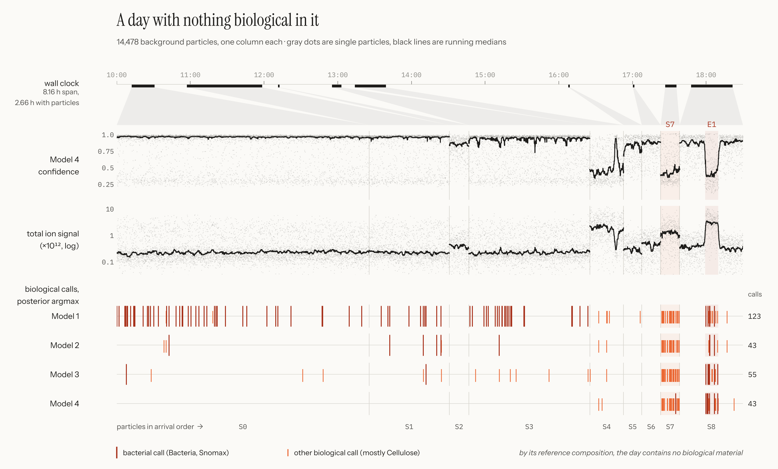 Figure 3: The background day, one column per particle. The top strip maps wall-clock time onto particle order, so dead time collapses out. Gray dots are single particles and black lines are running medians. Ticks mark each model’s biological calls (posterior argmax); dark ticks are bacterial calls, light ticks are other biological classes, mostly Cellulose. S7 is the low-confidence, high-ion segment; E1 is the late window where every model makes bacterial calls.
By lab standards, soot and cellulose are solved problems for these models. The Mean Teacher classifies all 14 laboratory soot particles correctly, and 95 of the 97 particles it calls Cellulose really are Cellulose. Then look at the segment of the day labeled S7 in Figure 3: 440 particles over about nine minutes of sampling. In S7 the Mean Teacher’s median confidence drops to 0.40, from roughly 0.95 earlier in the day, and 27 of its 43 biological calls for the entire day land there, 26 of them Cellulose. That is 6.1% of S7’s particles called biological, against 0.11% everywhere else, a 54-fold elevation. All four models show the same spike. I am deliberately not naming the material in S7 until I can line its timing up against the chamber’s sampling log, but the shape of the failure is unambiguous: material the models cannot place gets absorbed into the nearest class they know, and here that class happens to be biological. This is the lab-to-field gap in a single measurement, and it is exactly the failure an interferent-rejection requirement is written to catch.
The obvious defense is a novelty detector: flag particles that look unlike anything in training and refuse to classify them. So I tested the two candidates every practitioner reaches for. Low softmax confidence separates S7 from the rest of the day reasonably well, with an area under the ROC curve of 0.78 for the Mean Teacher. The instrument’s own total ion signal, which knows nothing about any classifier, separates S7 almost as well (0.75), which tells you the confidence collapse reflects something physically different about these particles rather than a quirk of one network. Autoencoder reconstruction error, the reflexive choice for this job, does something worse than fail. For the Mean Teacher it scores 0.21, meaning S7 particles are reconstructed better than ordinary ones (median error 0.59 versus 1.84). It points the wrong way. If you had shipped reconstruction error as your interferent guard, it would have waved the problem segment through with more confidence than the clean background.
The Hours You Can’t Tune Away
Two hard walls sit underneath every number above, and neither one cares how good your classifier is.
The first is observation time. If you watch a clean background for 2.66 hours and see zero alarms, the most you can claim at 95% one-sided confidence is a rate below 27 per 24 hours. Certifying the one-per-day requirement takes far more patience than most acceptance test plans budget for:
| Target rate (per 24 h) | Hours needed, 0 alarms allowed | 1 alarm allowed | 2 alarms allowed |
|---|---|---|---|
| 1 | 72 | 114 | 151 |
| 5 | 14 | 23 | 30 |
| 10 | 7 | 11 | 15 |
That is three full days of verified clean background with not a single alarm, or nearly five if you allow one. No threshold sweep substitutes for those hours, and a team that tunes its operating point on a short background and then reports the resulting rate as compliant has measured its own optimism.
The second wall is counting statistics on the detection side, and it surprised me. To measure detection probability, I spliced held-out laboratory bacterial particles into the real background stream at controlled arrival rates, in 1,000 simulated releases. At 0.2 agent particles per second, the probability of an alarm within 10 seconds came out at 0.88 for all four models, identical to two decimal places. The reason is that every model flags all 147 held-out bacterial particles at that threshold, so the classifier is not the bottleneck. Arrival is. With 0.2 particles per second you expect two agent particles in 10 seconds, and the chance that at least one shows up at all is . Meeting 90% within 10 seconds requires , or an agent arrival rate of at least about 0.23 particles per second at the inlet, no matter how good the model is. Persistence rules, which rescued the false-alarm numbers, make this worse: requiring two particles within 10 seconds drops detection to 0.62. Across every model, rule, and threshold I tested at that release rate, nothing reached 90% within 10 seconds. The trade between the two walls is the real design problem, and it is set by particle counting, not by architecture.
These detection numbers deserve their caveats stated plainly. The injected particles are laboratory library particles, so a fielded agent with a messier spectrum will score lower. Two of the four models used the development set in training decisions (a learning-rate scheduler and a checkpoint flag), so their detection numbers carry a small optimistic bias; the two SVMs are a clean holdout.
Closing Thoughts
The lesson I took from this is not that one of my models is better. It is that the question “which classifier is most accurate?” is the wrong question for anyone who has to field one. The right questions are how many particles per day the instrument sees, what per-particle error rate that implies, which alarm rule turns scattered errors into fewer events, what the system does with material it has never seen, and how many hours of clean background you need before you are allowed to claim anything. Each of those is answerable, and none of them shows up in a confusion matrix.
The benchmark is built so that any classifier that outputs per-particle posteriors can be dropped into it: a new score definition or a new alarm rule is a configuration change, and every output carries its interval. What it does not yet have is a second background day, a pollen-bearing background, or a field instrument, and that is where I need help. If you build particle sensors, work on bioaerosol triggers, run an indoor air quality practice, or model air quality for a state agency, I would like to hear what you would need added before a benchmark like this was useful to you. That answer is worth more to me than another decimal of lab accuracy, because a classifier is only as good as the number of times it cries wolf on a quiet day.
The background day is the FIN-01 blind sampling period (Shen et al., 2024), with PALMS spectra archived alongside Christopoulos et al. (2018); the classifiers come from my semi-supervised aerosol classification work. The benchmark code and derived model outputs are available upon request.