The Virtual Cook, Rebuilt

A Python reproduction of a 1999 cooking model, and the choices hidden inside its doneness score.

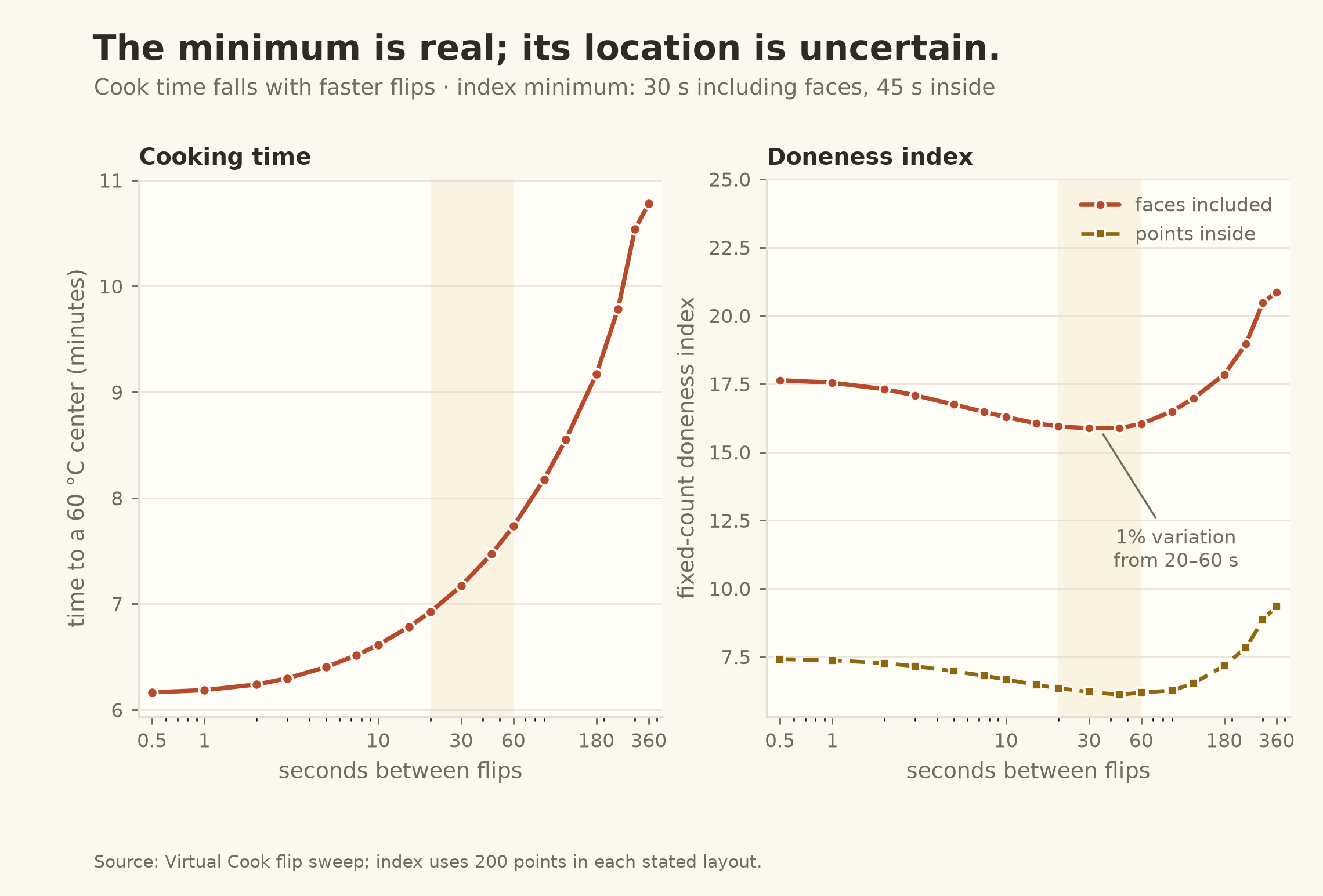
How often should you flip a burger? McGee et al.’s 1999 model puts the shallow minimum in its doneness index near a $15\,\mathrm{s}$ flip interval. My reproduction finds the minimum at $30\,\mathrm{s}$ when boundary points count and $45\,\mathrm{s}$ when only interior points count. Across $20$ to $60\,\mathrm{s}$ , though, the index changes by only about $1\%$ . The reversal is clear; a single best interval is not. These are simulation results at a $60^{\circ}\mathrm{C}$ center.

Doneness index versus flip interval, showing a shallow minimum whose location depends on the sampling convention. — *Figure 1: Faster flipping shortens the cook, while the shallow index minimum shifts from $30\,\mathrm{s}$ to $45\,\mathrm{s}$ with the sampling convention.*

The Model

In their 1999 Physics Today paper, McGee, McInerney, and Harrus treated a hamburger as a uniform, axisymmetric disk, $10\,\mathrm{cm}$ across and $2\,\mathrm{cm}$ thick, initially at $10^{\circ}\mathrm{C}$ . Fourier’s law, $\mathbf{q}=-k\nabla T$ , leads to the heat equation for this constant-property model:

\rho C\,\frac{\partial T}{\partial t}=\nabla\cdot(k\nabla T)

In boiling water, a heat-transfer coefficient of $10{,}000\,\mathrm{W/(m^2\cdot K)}$ gives a Biot number of $222$ and keeps the surface within $0.84^{\circ}\mathrm{C}$ of the bath, so a fixed-temperature boundary is a good approximation. For frying, the pan-facing surface is clamped at $100^{\circ}\mathrm{C}$ , while the off-heat face and the cylindrical rim lose heat to $20^{\circ}\mathrm{C}$ air through a Robin boundary with $h=20\,\mathrm{W/(m^2\cdot K)}$ . Each flip swaps the conditions on the two broad faces. Every simulation stops when the center reaches $60^{\circ}\mathrm{C}$ , the paper’s comparison point.

For this reproduction, I use fixed working inputs for lean beef: conductivity $0.45\,\mathrm{W/(m\cdot K)}$ , density $1050\,\mathrm{kg/m^3}$ , and specific heat $3500\,\mathrm{J/(kg\cdot K)}$ . Together they give a thermal diffusivity of $1.2245 \times 10^{-7}\,\mathrm{m^2/s}$ . These are project assumptions carried over from the series-plan toy case, not values reported by McGee et al.; the calculation holds them constant as the meat heats.

Temperature alone does not capture the paper’s idea of doneness, so the authors add a thermal-history score. Above $55^{\circ}\mathrm{C}$ , a quantity called $T^*$ doubles for every $10^{\circ}\mathrm{C}$ rise; below that threshold it is zero:

T^* = \begin{cases} 2^{T/10} & T \ge 55^{\circ}\mathrm{C} \\ 0 & T < 55^{\circ}\mathrm{C} \end{cases}

The model integrates $T^*$ through time at $200$ points in the disk’s central cross-section, sums those histories, and divides by $10^6$ . That final number is a sum over sampled points, not an average over the meat. The distinction will matter when we ask whether a reproduction gets the same answer.

Doneness index across three immersion bath temperatures, with the minimum at 70 degrees Celsius. — *Figure 2: The doneness index falls as the bath cools from $100^{\circ}\mathrm{C}$ to $70^{\circ}\mathrm{C}$ , then reaches its minimum at $70^{\circ}\mathrm{C}$ .*

Can the Model Reproduce the Paper?

For the $2\,\mathrm{cm}$ disk immersed in a $100^{\circ}\mathrm{C}$ bath, the reproduction gives a doneness index of $24.5$ ; the paper reports $23.0$ . At $80^{\circ}\mathrm{C}$ , the two values are $10.3$ and $10.2$ , and at $70^{\circ}\mathrm{C}$ both are $8.1$ . The lowest score still falls at $70^{\circ}\mathrm{C}$ . The model recovers the pattern, while its absolute index is a little higher.

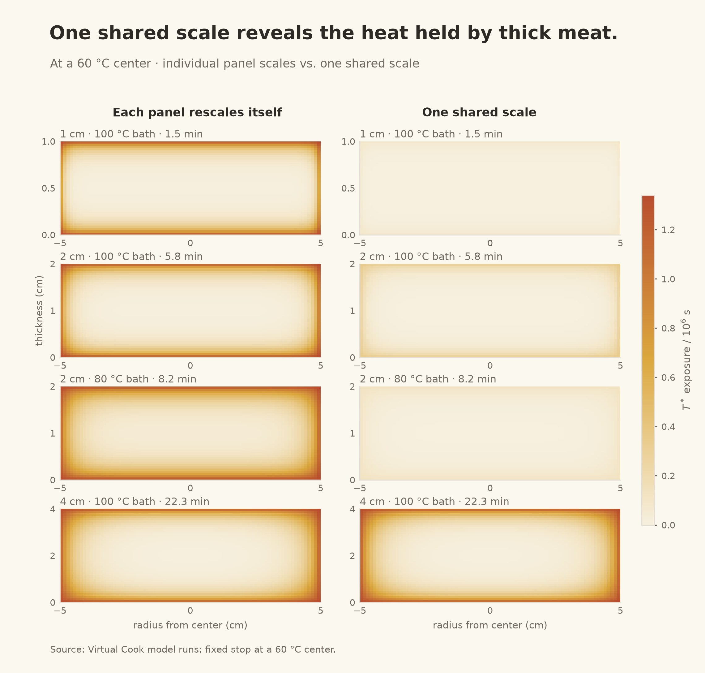
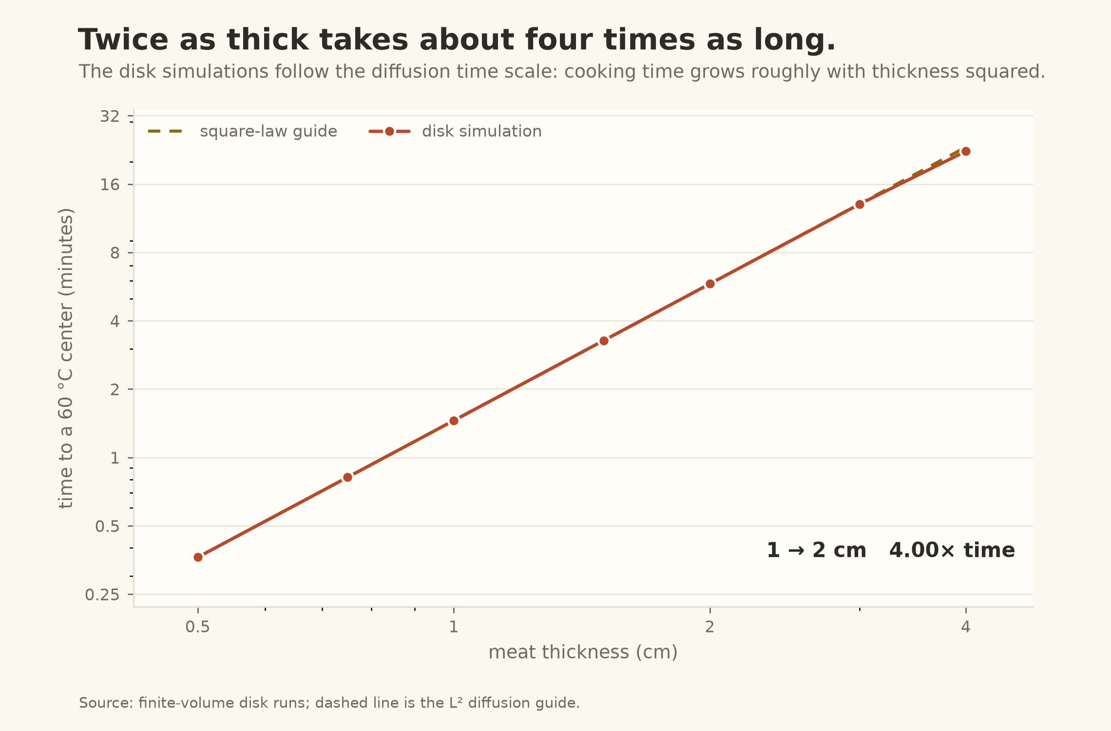
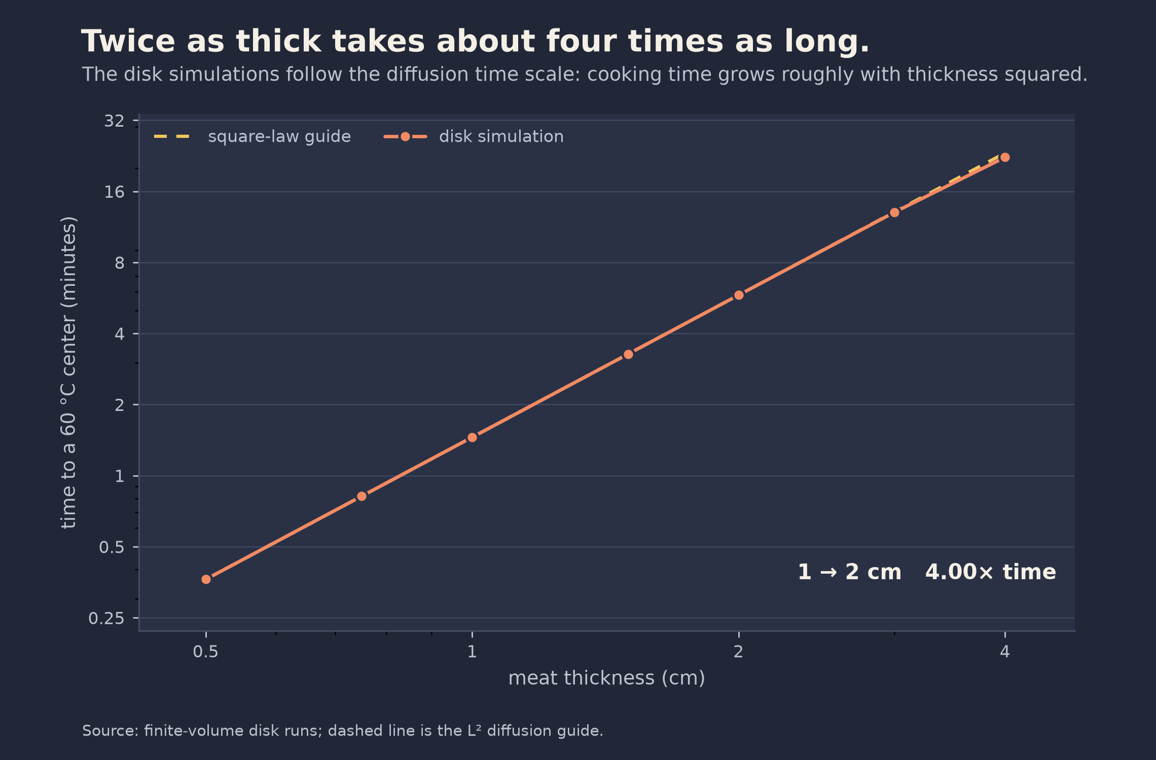
Other checks land close to their reported targets. For a $1\,\mathrm{cm}$ disk in a $100^{\circ}\mathrm{C}$ bath, the model’s $\pm5^{\circ}\mathrm{C}$ center-temperature window lasts $19.5\,\mathrm{s}$ , compared with $20\,\mathrm{s}$ in the paper, and its center warms at $29.3^{\circ}\mathrm{C/min}$ rather than $30^{\circ}\mathrm{C/min}$ . A one-dimensional slab gives another check: separation of variables yields an exact temperature profile, and the solution depends on the Fourier number, $Fo = \alpha t/L^2$ , so the time to the same center temperature scales with thickness squared. For the $10^{\circ}\mathrm{C}$ start and $100^{\circ}\mathrm{C}$ bath, the slab reaches a $60^{\circ}\mathrm{C}$ center at $Fo \approx 0.1066$ , giving $1.45\,\mathrm{min}$ at $1\,\mathrm{cm}$ , $5.81\,\mathrm{min}$ at $2\,\mathrm{cm}$ , and $23.22\,\mathrm{min}$ at $4\,\mathrm{cm}$ . The 2D disk runs show the same penalty: a $1\,\mathrm{cm}$ disk takes about $1.5\,\mathrm{min}$ , while a $4\,\mathrm{cm}$ disk takes $22.3\,\mathrm{min}$ . The 2D disk cooks slightly faster than the slab at $4\,\mathrm{cm}$ because heat also enters through its rim.

Cooking time rises with disk thickness; doubling thickness gives four times the cooking time. — *Figure 3: Doubling the distance heat travels gives a fourfold increase in cooking time.*

Before trusting the disk simulations, I compare the finite-volume solver with exact one-dimensional slab solutions for fixed-temperature and convective boundaries. Those analytical profiles give a known answer against which to check the numerical method before applying it to the axisymmetric disk. Across five grid refinements, the spatial error falls at second order; after a boundary flip, two backward-Euler steps damp the surface ringing from Crank–Nicolson while preserving second-order temporal convergence. The energy imbalance in these checks ranges from $10^{-14}$ to $10^{-12}$ . The cooking runs use a $40\times41$ axisymmetric mesh and $0.1\,\mathrm{s}$ time steps, with the reported quantities within about $0.5\%$ of their mesh-converged values. These checks support the numerical method, but they cannot decide how the paper’s index should count sample points.

A Warmer Start, a Faster Cook

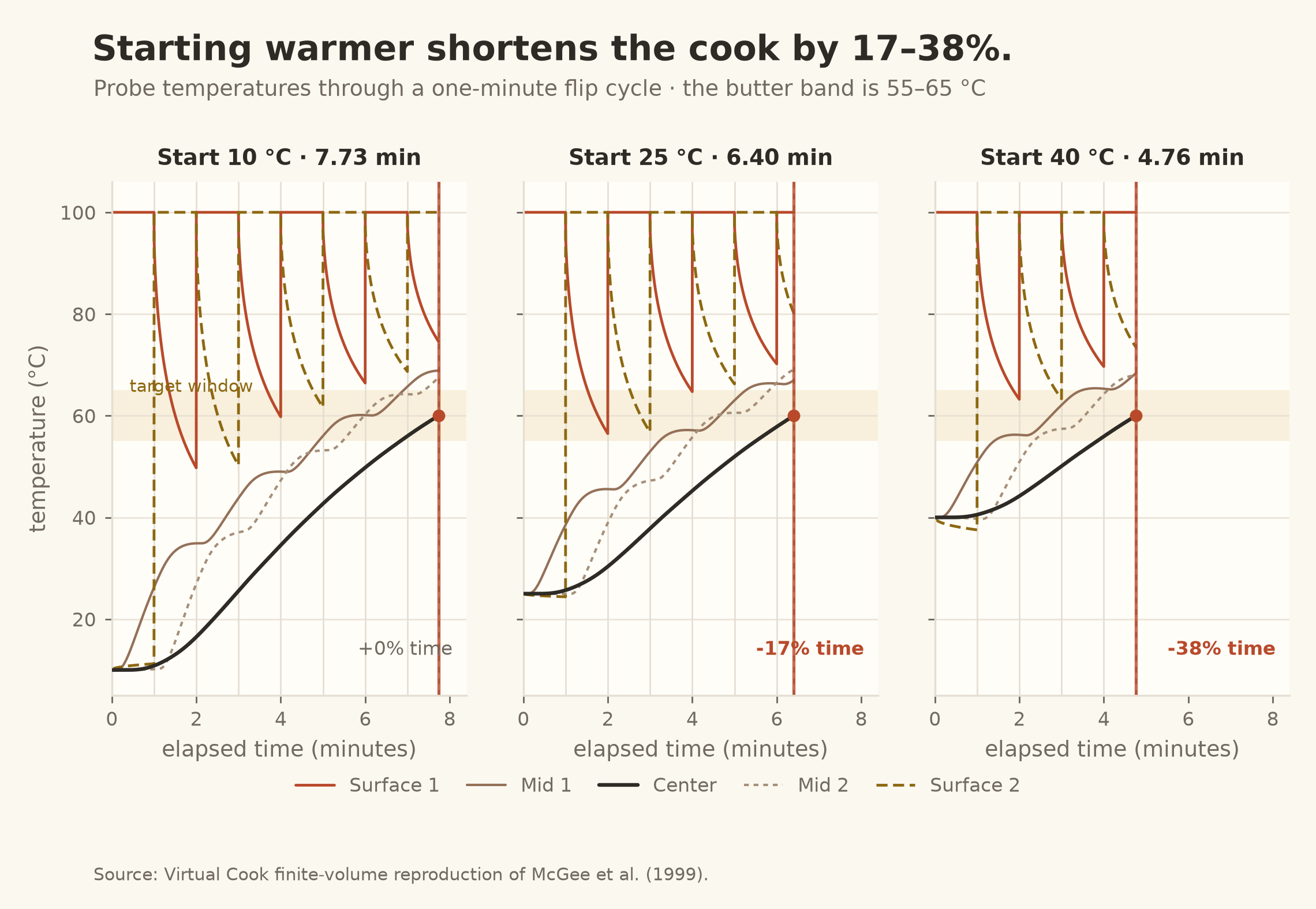
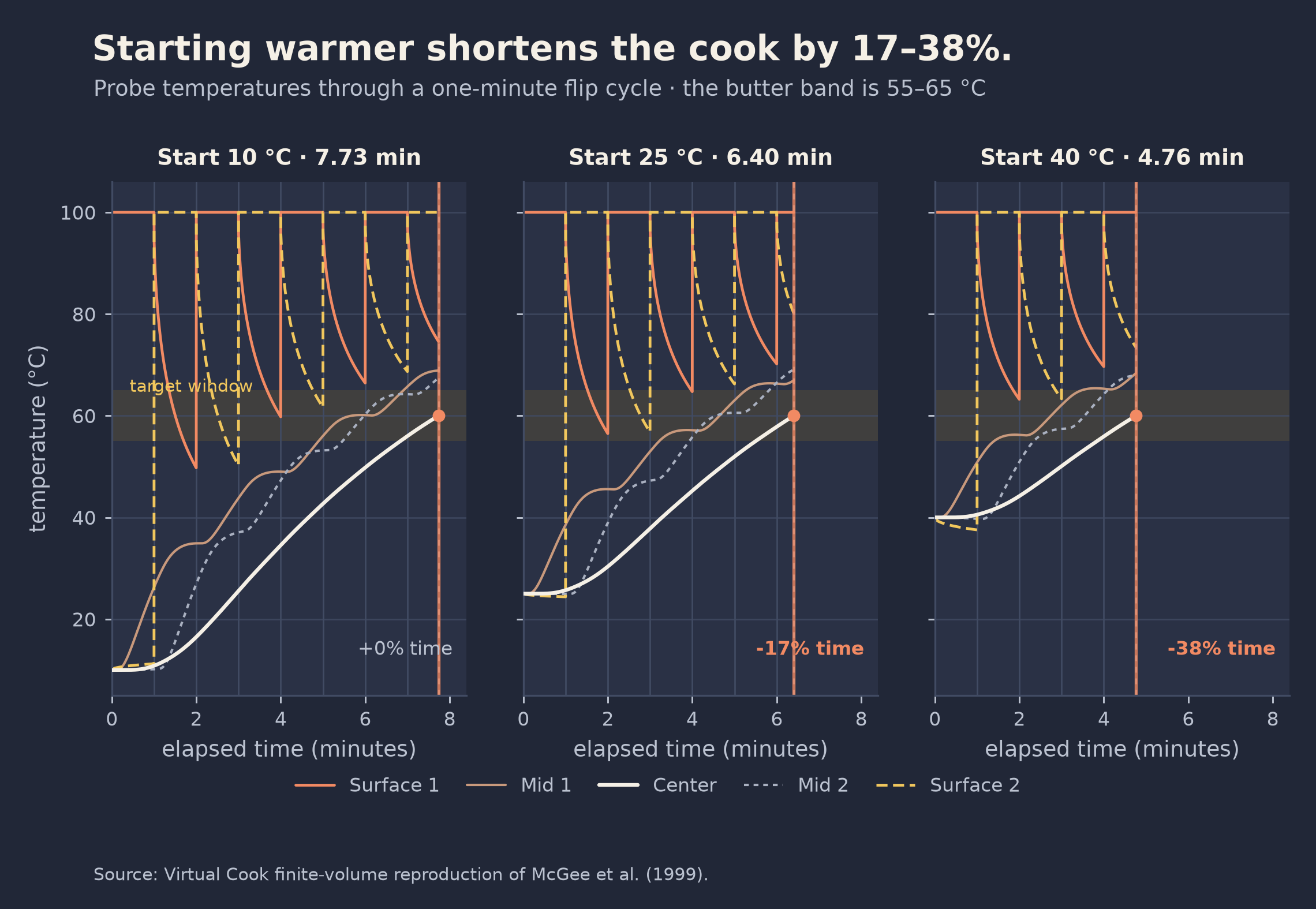
The bath and the disk’s thickness are not the only ways to change the time to a $60^{\circ}\mathrm{C}$ center. Begin with the same $2\,\mathrm{cm}$ disk at $10^{\circ}\mathrm{C}$ , then raise its starting temperature before cooking: prewarming it to $25^{\circ}\mathrm{C}$ shortens the cook by $17.2\%$ , while starting at $40^{\circ}\mathrm{C}$ shortens it by $38.5\%$ . The hotter start gives heat less ground to cover before the center reaches its target. That change in cooking time is direct and easy to interpret.

The doneness index shifts too, but its size depends on how the sample points are counted. At $25^{\circ}\mathrm{C}$ , it falls by $14.0\%$ with boundary points included and by $8.6\%$ with interior points alone; the paper reports about $8\%$ . At $40^{\circ}\mathrm{C}$ , cooking time falls by $38.5\%$ , while the index falls by $33.7\%$ under the boundary-inclusive convention. The time comparison follows the temperature field; the index comparison also inherits the rules used to sample it. A warmer start changes both the cook and the score, but the score is the less portable measure.

Cooking time decreases as the disk's initial temperature rises from 10 to 25 and 40 degrees Celsius. — Figure 4: Raising the initial temperature from $10^{\circ}\mathrm{C}$ to $25^{\circ}\mathrm{C}$ or $40^{\circ}\mathrm{C}$ shortens the time to a $60^{\circ}\mathrm{C}$ center by $17.2\%$ or $38.5\%$ .

What Does Flipping Change?

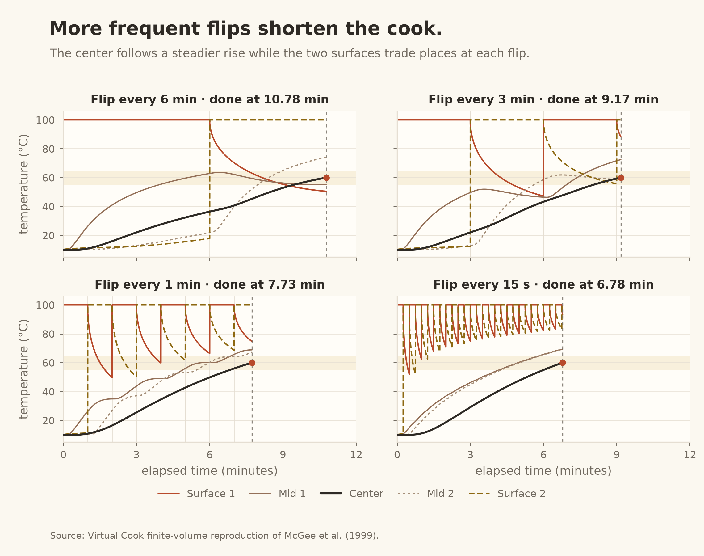
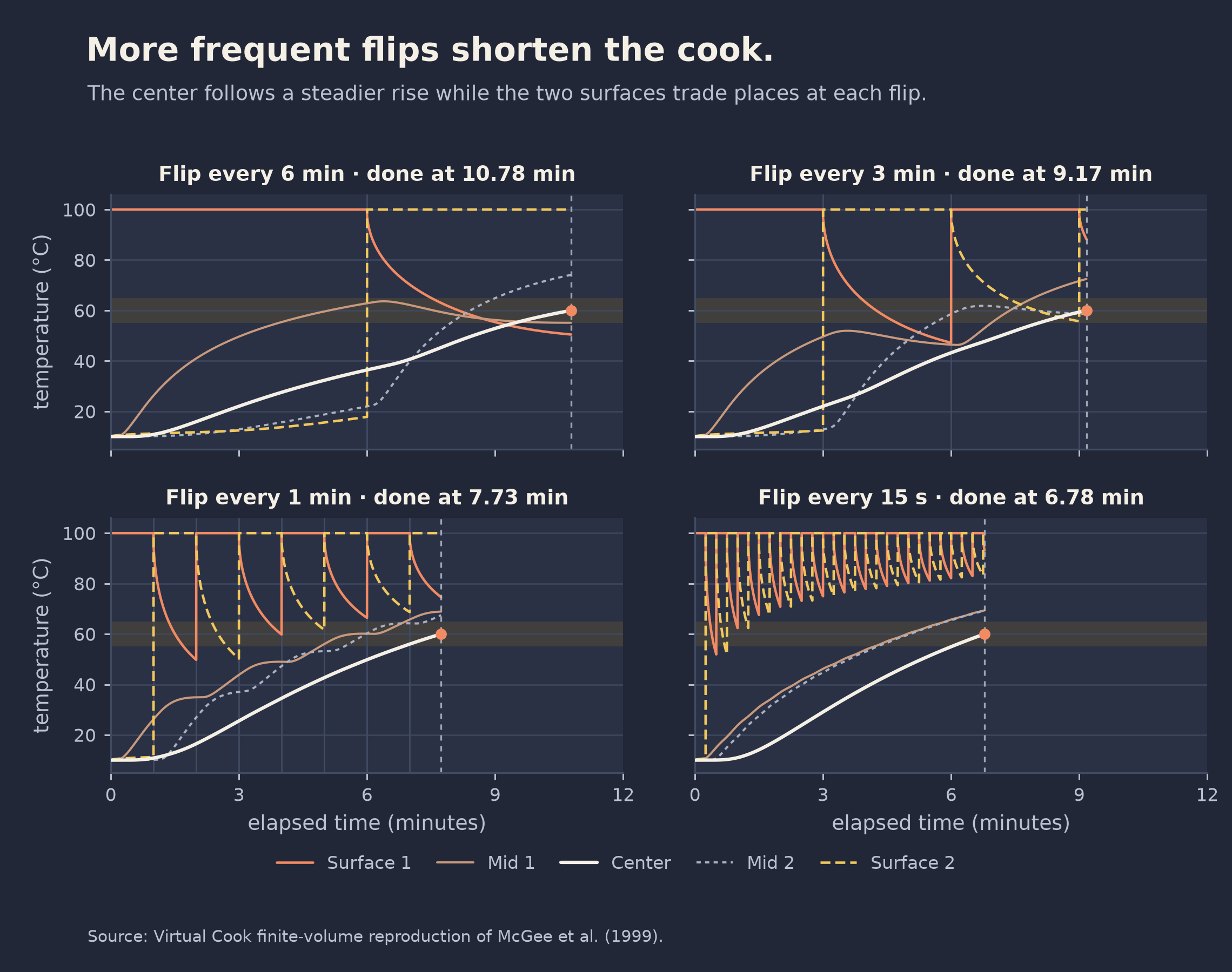
In the frying cases, one face contacts the hot pan while the other faces the air, and the two conditions exchange when the disk flips. With a $6\,\mathrm{min}$ interval between flips, the center reaches $60^{\circ}\mathrm{C}$ in $10.78\,\mathrm{min}$ . Flipping every $1\,\mathrm{min}$ brings that time down to $7.73\,\mathrm{min}$ . The heating surface alternates more often, so the center warms sooner. More frequent flipping speeds this cook.

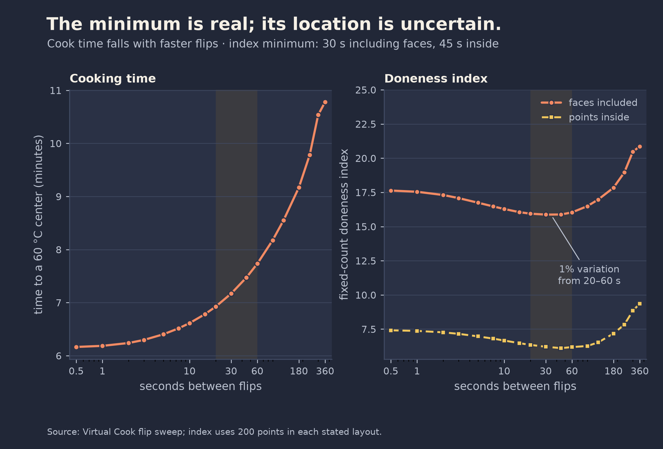
The paper’s more surprising claim concerns the doneness index, which has a shallow minimum near a $15\,\mathrm{s}$ flip interval. The reproduction also finds a shallow minimum, but its sampled location is $30\,\mathrm{s}$ when the cooking faces are included and $45\,\mathrm{s}$ when only interior points are counted. Across intervals from $20\,\mathrm{s}$ to $60\,\mathrm{s}$ , the score changes by about $1\%$ . The direction of the curve survives; its precise minimum does not.

Temperature profiles for frying cases with six-minute and one-minute flipping intervals. — *Figure 5: Temperature histories at five depths for flip intervals of $6\,\mathrm{min}$ , $3\,\mathrm{min}$ , $1\,\mathrm{min}$ , and $15\,\mathrm{s}$ .*

The Index Has a Counting Problem

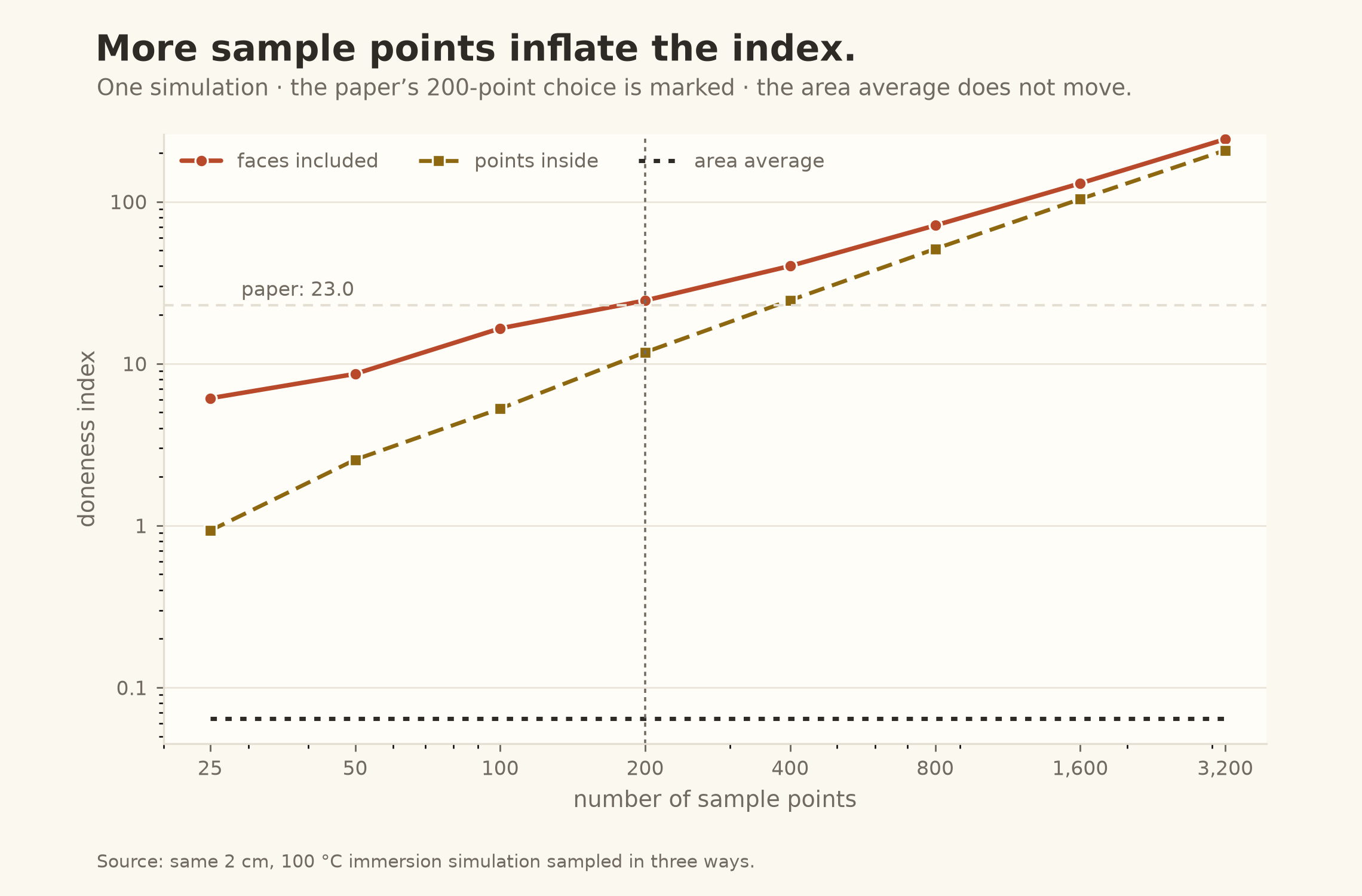
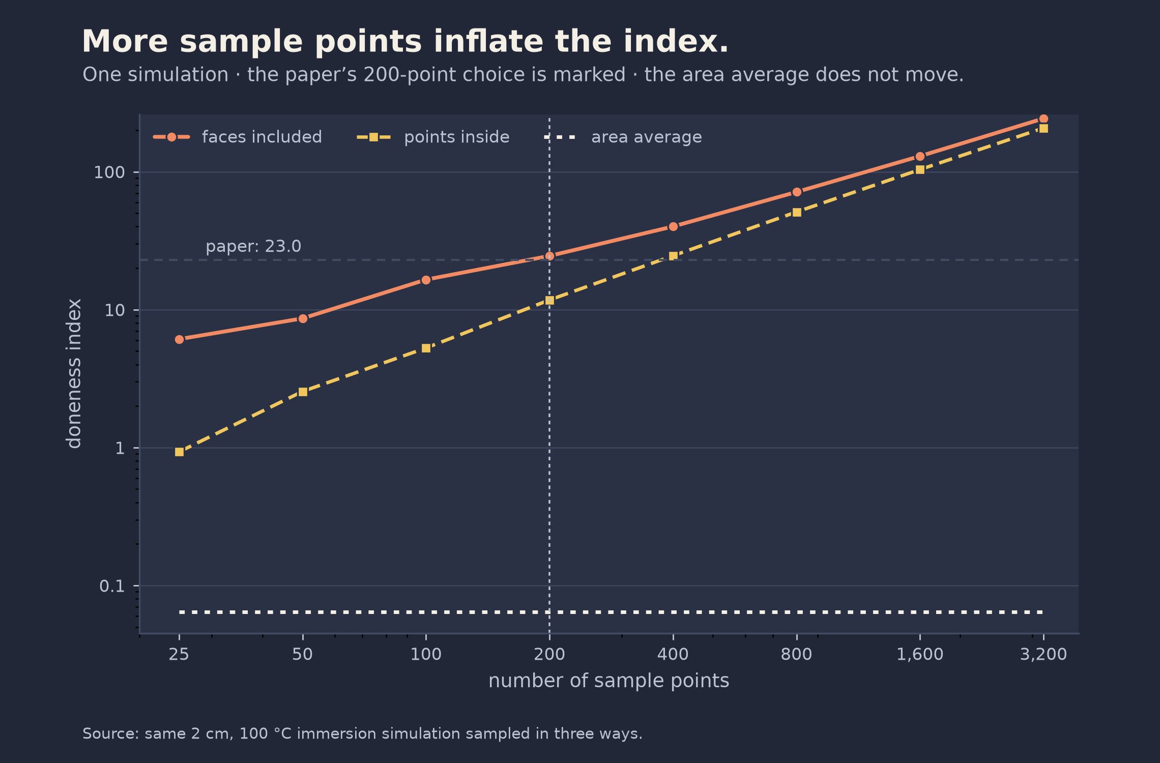
The paper’s index adds the integrated thermal history at each sample point and divides by a fixed constant. If the same temperature field is sampled more densely, the sum grows: on this run, increasing the grid from $200$ points to $3200$ raises the index from $24.52$ to $243.03$ , nearly tenfold. The area average stays at $0.0642$ . The sum measures how many points were counted as well as how much of the meat was cooked.

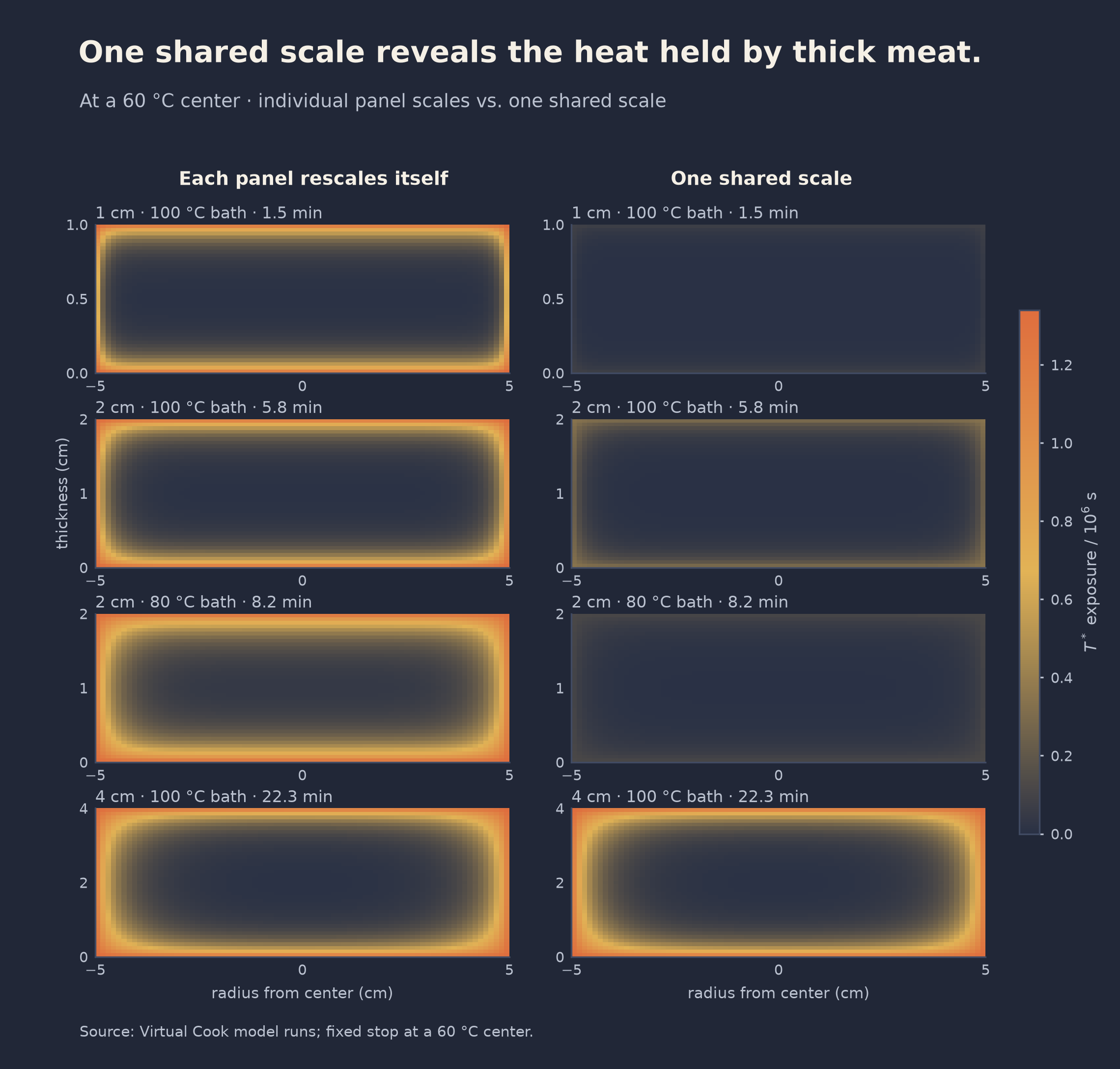
Where those points sit changes the answer too. With $200$ points, including the two cooking faces gives $24.5$ ; using only points strictly inside the meat gives $11.7$ for the same simulation. The faces remain at the $100^{\circ}\mathrm{C}$ bath temperature, where $T^*$ is $1024$ , compared with $64$ at the $60^{\circ}\mathrm{C}$ center. As a result, $50$ face samples contribute $73\%$ of the sum, while the $144$ interior samples contribute $18\%$ .

This choice also changes the apparent location of the flip-interval minimum, even though the simulated temperature fields are identical. The boundary-inclusive convention gives ratios of $2.37$ for the $100^{\circ}\mathrm{C}$ -to- $80^{\circ}\mathrm{C}$ bath comparison and $3.03$ for the $100^{\circ}\mathrm{C}$ -to- $70^{\circ}\mathrm{C}$ comparison, compared with the paper’s $2.26$ and $2.84$ ; the interior-only convention gives $1.77$ and $1.95$ . That is evidence that the paper included boundary points, though it cannot prove the original grid layout. The prewarming comparison is a useful counterexample: its $25^{\circ}\mathrm{C}$ index change is closer to the paper under interior-only sampling. I report the area average beside the paper-style sum so a reader can see both and compare the result across meshes.

The paper-style doneness index changes with sample count and point placement, while the area average remains stable. — *Figure 6: The paper-style index grows with sample count and nearly halves when face points are omitted; the area average is stable.*

Conclusion

Rebuilding the virtual cook recovers the paper’s main comparisons: cooler immersion baths lower the index, doubling thickness quadruples cooking time, and frequent flipping brings the center to its target sooner. It also exposes a less visible choice inside the headline score. The solver can be refined and checked, but a sum over an unspecified set of points will still depend on how those points are chosen.

The next useful step is to replace that sum with a spatial average and keep the original convention alongside it when comparing with the paper. One target remains outside this reproduction: the spit-roast case needs a three-dimensional model with a rotating radiative boundary. The next post will relax the assumption that every part of the meat has the same properties, and ask how internal variation changes cooking time. For the burger in the bath, the distance heat must travel still explains the long wait. The counting rule explains why the score is harder to trust.

Part of my research notes on heat transfer in cooking. Based on McGee, McInerney, and Harrus, “The Virtual Cook: Modeling Heat Transfer in the Kitchen,” Physics Today 52(11), 30–36 (1999); numerical results are from the Post 1 reproduction notebook.