The Unlabeled Data Didn’t Help
Mean Teacher against a control that shares everything except the idea
You have a classifier that works. It sorts single-particle mass spectra of atmospheric aerosols into 20 classes (mineral dusts, agricultural soils, feldspars, biological particles, soot, secondary organics) from 194 mass peaks per particle. You also have a pile of spectra nobody has labeled, and a semi-supervised method that promises to turn that pile into accuracy. You try it, it wins, and you write it up. That’s what happened in the original version of this project: Mean Teacher was the best model we had, ahead of the supervised baselines. When I rebuilt the whole pipeline from scratch with a stricter protocol, the win was still there. It just didn’t belong to the unlabeled data.
This post is about how I found that out, and why the comparison that found it is the part I’d keep even if every number changed.
The Promise of Unlabeled Data
Mean Teacher is one of the cleanest ideas in semi-supervised learning. You train a normal network, the student, on the labeled data. Alongside it you keep a second copy, the teacher, whose weights are an exponential moving average (EMA) of the student’s weights over training. The teacher never takes a gradient step; it is a smoothed, slightly delayed version of the student. Then, on every batch, you show both networks the same spectra with independent random noise added, including spectra that have no labels, and you add a consistency loss that penalizes the student when its predicted class probabilities disagree with the teacher’s. The labels teach the student what the classes are. The consistency term teaches it to give the same answer to a particle whether or not its peaks are jittered, everywhere in the input space the unlabeled data covers.
The intuition is a bit like learning a language from a tutor plus a lot of overheard conversation. The tutor (labels) corrects you directly; the conversation (unlabeled data) never tells you what’s right, but it shows you which sounds tend to go together, and it punishes you for interpreting the same sentence two different ways. If labels are expensive and unlabeled spectra are cheap, that second source of signal should be worth something.
It’s worth stating the scale up front, because it matters later. After the outlier rule (drop spectra with fewer than two nonzero peaks) the labeled set holds 18,678 spectra, and the unlabeled pool holds 14,478. This is not a regime where labels are scarce. The unlabeled pool is actually smaller than the labeled set.
The Recipe Is Not the Idea
Here’s the trap. Mean Teacher is never just the consistency loss. To run it you change a lot of things at once: every batch becomes a mix of labeled and unlabeled spectra, the inputs get random noise, the model you keep at the end is the EMA teacher rather than the raw student, and the training schedule changes because the consistency weight ramps up over the first few dozen epochs. Any one of those can make a network better on its own. Noise injection is a regularizer. Weight averaging is a regularizer. If you compare Mean Teacher against a plain supervised network, you are comparing a whole recipe against no recipe, and the unlabeled data gets the credit for everything.
So the rebuild has a matched control: the same training function, the same mixed batches drawn from the same unlabeled pool, the same input noise, the same EMA teacher, the same rule for picking the checkpoint (teacher at its best validation macro-F1), with exactly one change. The consistency weight is set to zero. The unlabeled spectra still flow through the batches, but nothing ever reads a prediction on them. The two arms differ only in the one term that makes Mean Teacher semi-supervised.
Both arms were tuned with the same budget and the same protocol: Bayesian optimization over the shared hyperparameters (learning rate, batch size, EMA decay, noise level and kind, unlabeled fraction of each batch), plus the consistency-specific ones for Mean Teacher (weight, ramp length, loss type, confidence threshold). Finalists were rescored on five inner folds of a development set, and the configurations were frozen before anything touched a test fold. In the third rebuild the selected Mean Teacher used a KL-divergence consistency loss with weight 1.37 and a 35-epoch ramp, a teacher EMA decay of 0.974, and about half of each batch unlabeled. That is not a token amount of consistency. If the unlabeled data had something to say, this configuration was listening.
Each test fold was read exactly once. I ended up with three of them, because the rebuild went through three versions (v1 with untuned recipes, v2 tuned, v3 with a fix to how autoencoders were chosen), and every time I fixed something I carved a fresh fold rather than re-reading an old one. The three results are never pooled or averaged; they are three separate experiments that happen to ask the same question.
Three Folds, One Answer
Here is Mean Teacher minus its matched control, in test macro-F1, on each fold:
| test fold | spectra | Mean Teacher | matched control | difference |
|---|---|---|---|---|
| v1 (untuned) | 2,669 | 0.918 | 0.916 | +0.002 |
| v2 (tuned) | 2,669 | 0.920 | 0.918 | +0.0015 |
| v3 (tuned, fresh fold) | 2,742 | 0.925 | 0.930 | −0.005 |
The first two differences are tiny and positive. The third is small and negative. None of them is anywhere near the width of the 95% bootstrap intervals, which run about ±0.01 on every model. In v3 the comparison is about as clean as it gets: five reporting seeds per arm, and Mean Teacher is below the control on all five (0.926 vs 0.930, 0.923 vs 0.926, 0.928 vs 0.934, 0.926 vs 0.930, 0.922 vs 0.931). The development-set cross-validation had predicted the same thing before the test fold was opened, 0.926 for Mean Teacher against 0.927 for the control. The sign of the effect flips between folds and its size never escapes the noise. That is what “no effect” looks like.
What did help was the recipe. In v1, where I also trained a plain network with no mixed batches, no noise and no EMA, the control beat it by 0.006 and Mean Teacher beat it by 0.008. Almost all of the improvement that the original project attributed to semi-supervision was sitting in the scaffolding around it.
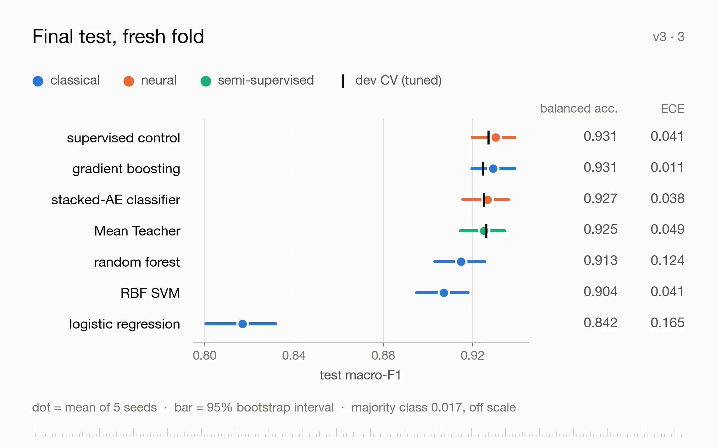
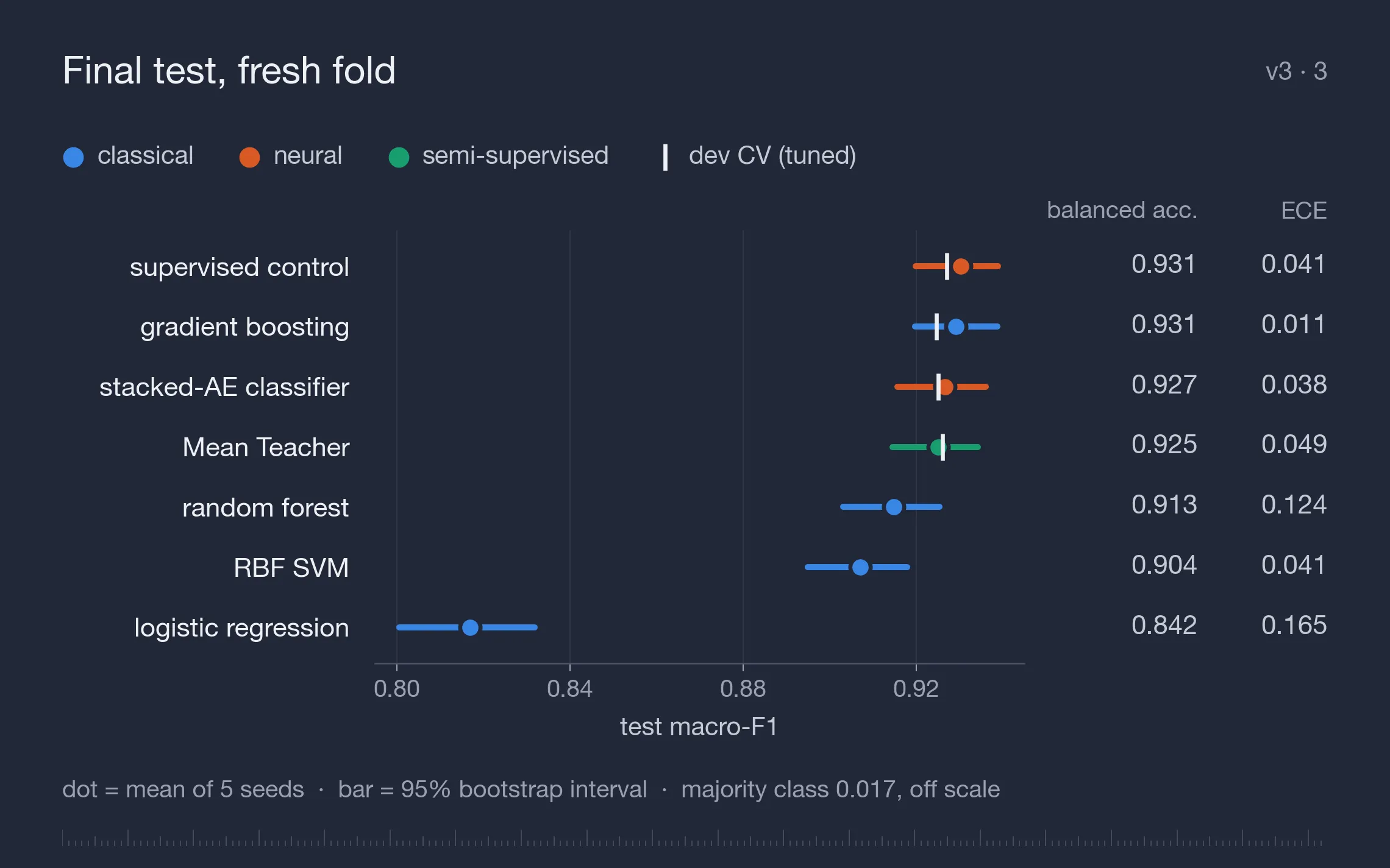
Figure 1: Test macro-F1 on the v3 fold of 2,742 spectra, read once. Dots are the mean over five seeds, bars are 95% bootstrap intervals over test particles, and black ticks are the five-fold development-set score of each tuned configuration. Right columns: balanced accuracy and expected calibration error (ECE, lower is better). The supervised control, gradient boosting, the stacked-autoencoder classifier and Mean Teacher overlap within their intervals.
What the Training Curves Show
The tuning runs didn’t originally save per-epoch histories, so I replayed the ten selected runs of each arm (five folds × two seeds) on the development set; the replays reproduce the original best scores and best epochs exactly. The curves tell a more interesting story than the final table.
Mean Teacher gets good fast. Averaged over the ten runs, its teacher reaches a validation macro-F1 of 0.901 by epoch 10 and 0.918 by epoch 20, while the control is at 0.878 and 0.902. But it doesn’t go higher. The best validation score averages 0.926 for Mean Teacher and 0.927 for the control; the control simply takes longer to get there, with best epochs between 41 and 108 against 20 to 104 for Mean Teacher. Both arms converge to the same ceiling.
It’s tempting to read that early lead as the unlabeled data speeding up learning. I don’t think the curves support it. By epoch 10 the consistency weight has only ramped to 0.09 (out of 1.37), so the consistency term is barely switched on when most of the gap opens. The two arms were tuned separately, and the selected Mean Teacher has a higher learning rate (0.0022 against 0.0013), which is a much more boring explanation for a faster start. The consistency loss itself does behave as designed: it falls from 0.13 to 0.05 over the first 40 epochs, and the fraction of samples that pass the teacher’s 0.5 confidence gate rises from 15% to about 95% in a typical run. The student learns to agree with the teacher. It just doesn’t learn anything the labels hadn’t already taught it.
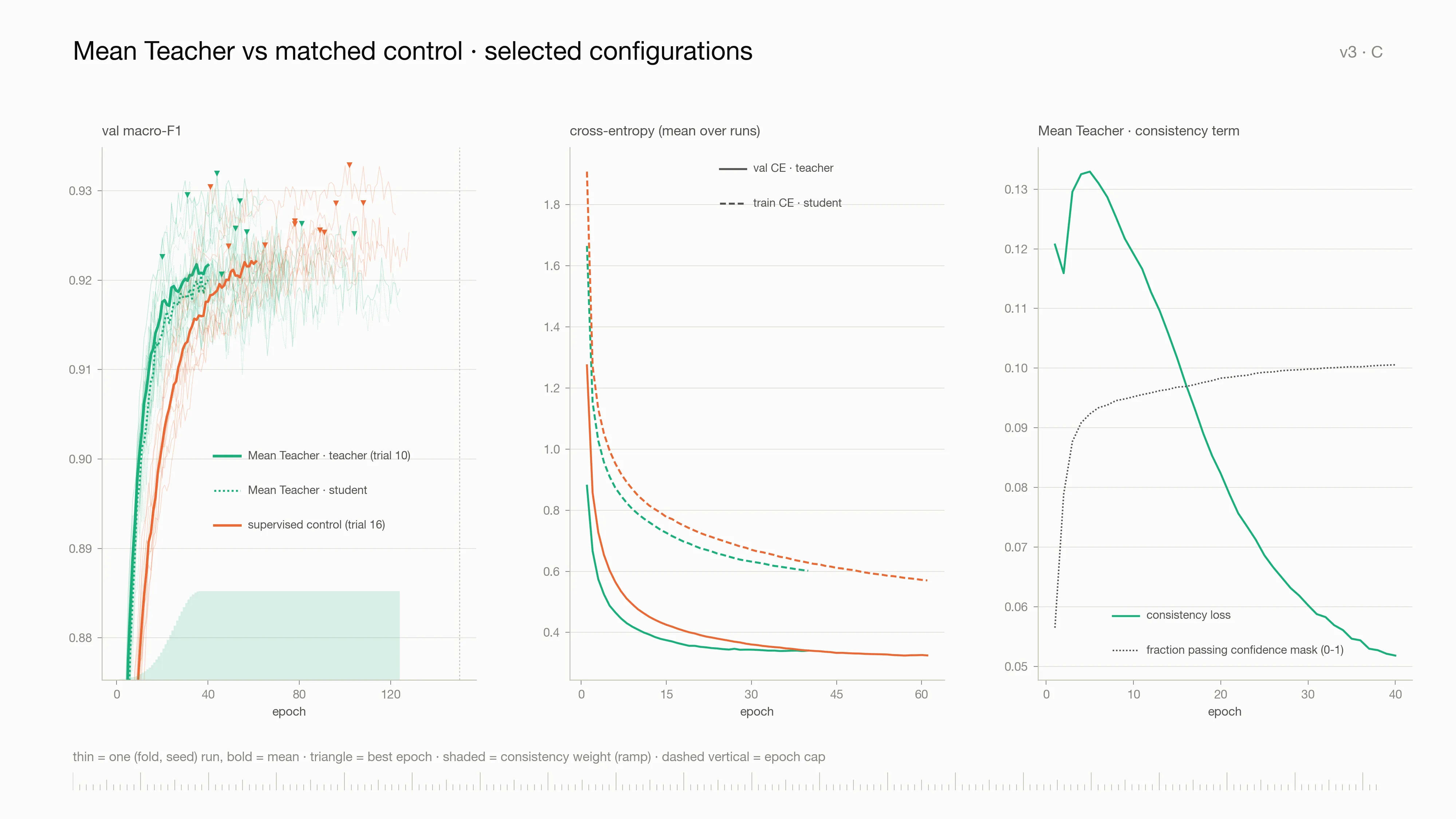
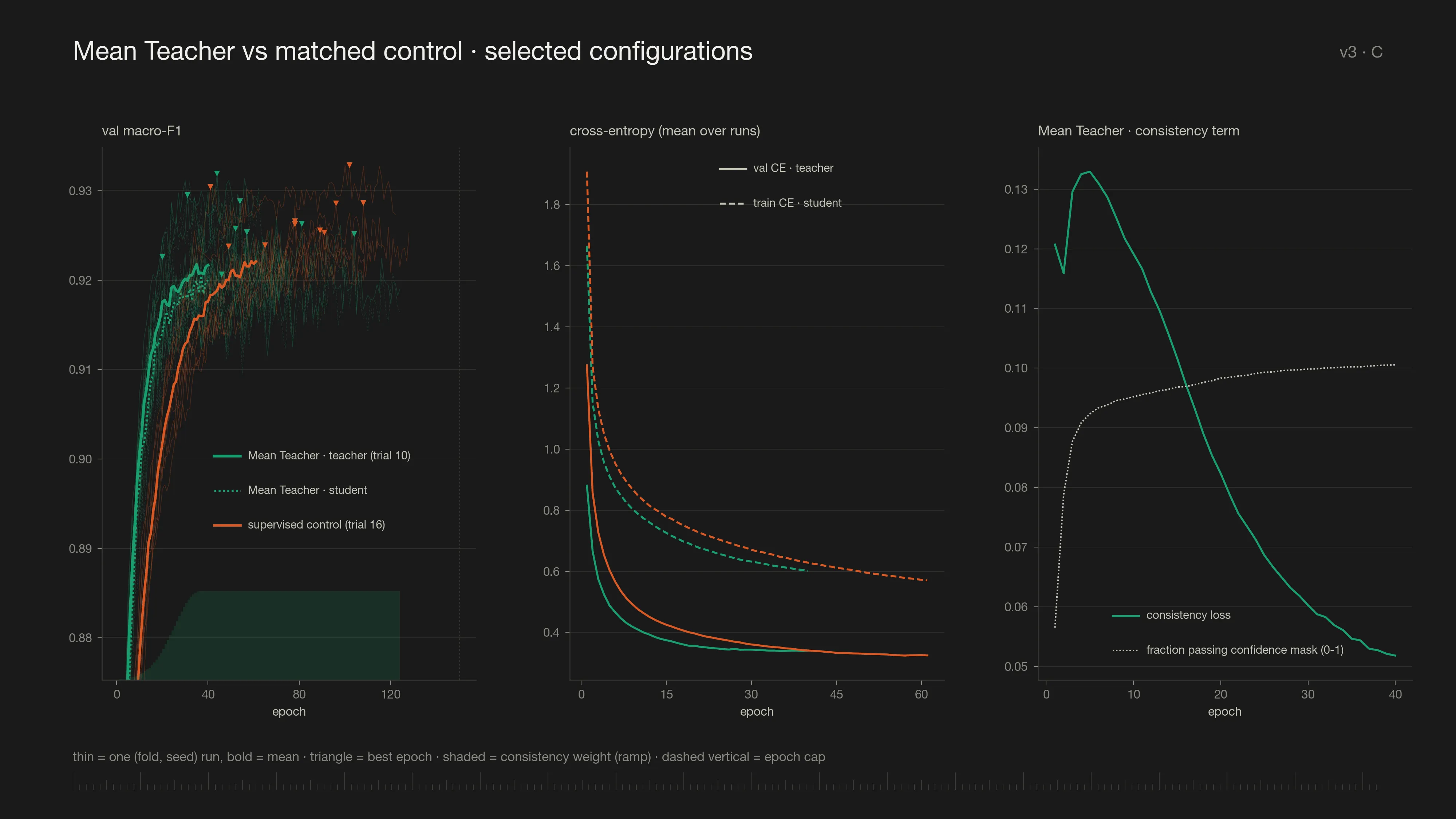
Figure 2: Training curves for the selected Mean Teacher (green) and matched control (orange) configurations, replayed on the development set. Left: validation macro-F1, thin lines are single (fold, seed) runs, bold lines are means, triangles mark best epochs, and the shaded band is the consistency weight ramp. Middle: cross-entropy. Right: the consistency loss and the fraction of samples passing the confidence gate. Click to enlarge.
The Boring Model in the Room
If the semi-supervised story deflates, the obvious follow-up is whether neural networks were needed at all. Gradient boosting on the raw peak vectors, with no pretraining, no unlabeled data and no GPU, scores 0.929 on the v3 fold, against 0.930 for the best neural model. Those are the same number for any practical purpose. Where gradient boosting clearly wins is calibration: its expected calibration error is 0.011, against 0.038–0.049 for the neural models. When it says it’s 90% confident, it’s right about 90% of the time. If those probabilities feed anything downstream, such as source apportionment or a threshold for flagging particles, that matters more than the third decimal of F1.
The per-class picture explains why everything ties. The hard classes are the same for every model: the four feldspars (Na, K, cSA, cSOA) and three agricultural soils (Argentinian, Chinese, German). Na Feldspar is the hardest class for all seven models, from 0.58 for logistic regression to 0.76 for the control, gradient boosting and the stacked autoencoder (Mean Teacher sits at 0.73). Classes like bacteria, Snomax and SOA sit near 1.00 for everyone. Among the tuned models, no class moves by more than about 0.03. Every model trips over the same particles, which says the difficulty lives in the spectra themselves, not in the choice of method. Feldspars with different cations and coatings simply produce very similar negative-ion spectra, and no amount of consistency regularization separates two classes that look the same.
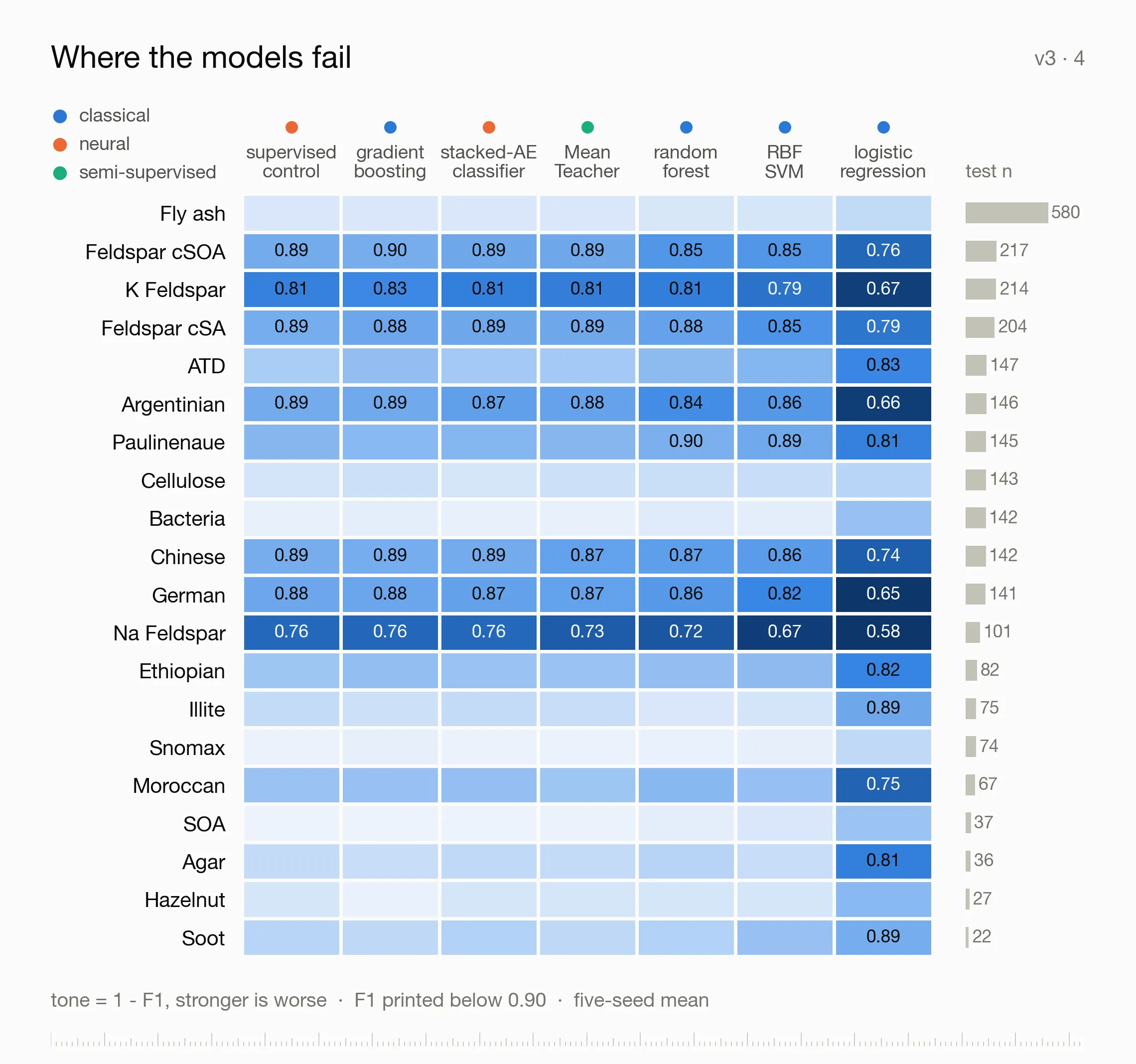
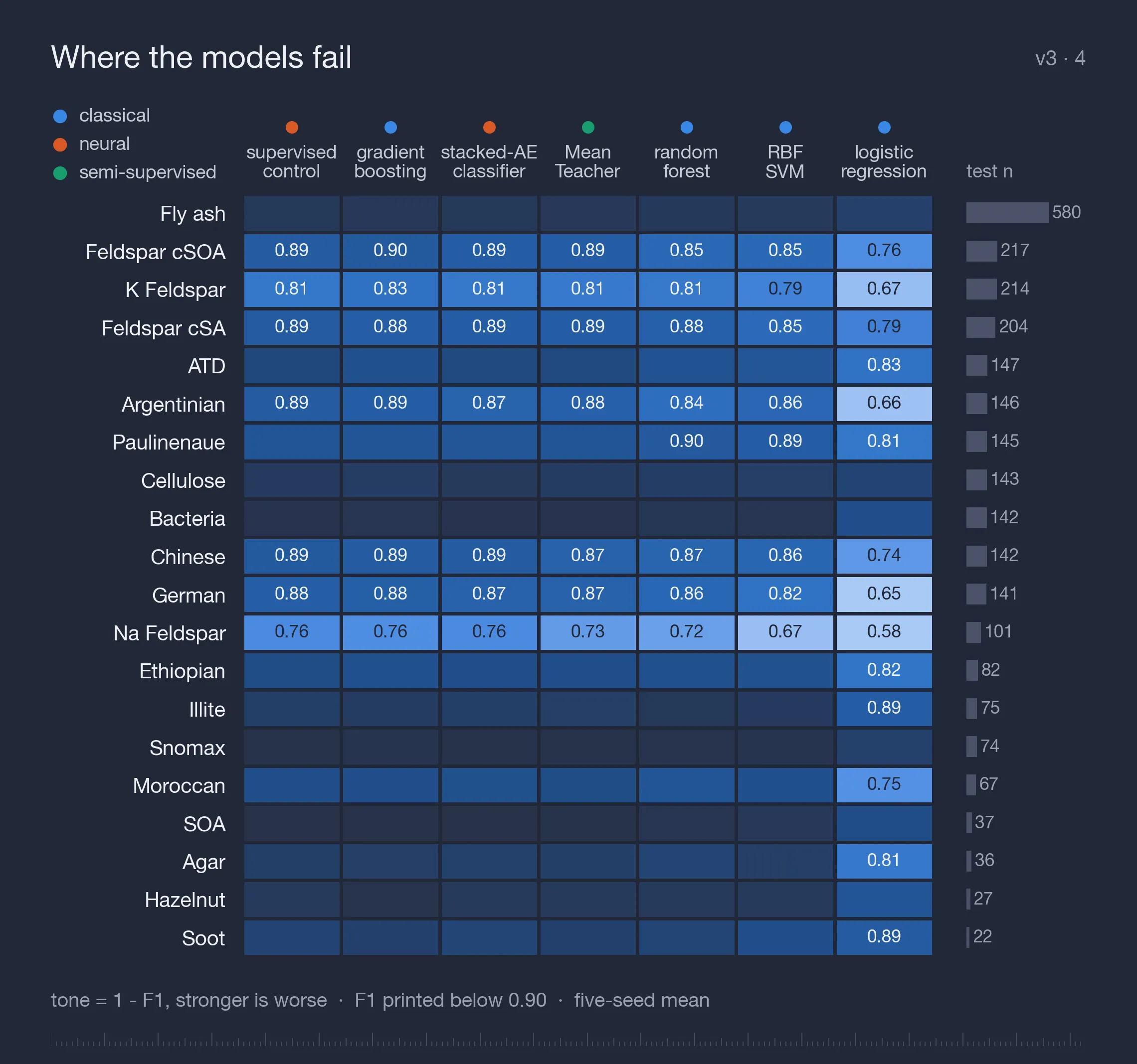
Figure 3: Per-class test F1 (five-seed mean) on the v3 fold. Rows are the 20 aerosol classes ordered by test support (bars, right); columns are the models ordered by test macro-F1. Darker cells are worse, and values are printed where F1 is below 0.90. The feldspars and agricultural soils are hard for every model.
Closing Thoughts
None of this says Mean Teacher is a bad method. It says that on this dataset, with this many labels, the unlabeled pool has nothing to add that 18,678 labeled spectra hadn’t already provided. That’s the regime where you’d expect semi-supervision to struggle, and in hindsight the scale alone should have made me suspicious. There are also limits to what this experiment can see. The splits are random and stratified, because the labeled particles carry no acquisition run or day IDs, so the test folds measure generalization to new particles from familiar sample sources. Identical spectra are grouped across splits, near-duplicates are not. And the unlabeled pool here is from the same instrument and setting as the labels; the case where unlabeled data should help most, adapting to ambient air that doesn’t look like the lab, is exactly the case this test can’t measure.
The practical lesson is about the comparison, not the method. Before you credit any technique with a gain, build the control that shares everything with it except the idea itself, give both the same tuning budget, and read the test fold once. If the gain survives, you’ve learned something about the idea. If it doesn’t, you’ve learned something about your recipe, which is often the more useful thing to know. Here, the control shared everything except the idea, and it turned out the idea wasn’t doing the work.
Part of my notes on rebuilding the SPMS aerosol classifier. Spectra are negative-ion single-particle mass spectra of laboratory aerosols (Christopoulos, Costa et al., 2018) plus an unlabeled pool from the same instrument. Code and results are available upon request.